Mentors
- Raghav Bajpai
- Aakanksha
- Nikesh shetty
Members
- Shubhankar Ghosh
- Dhanush
Acknowledgements
Would like to thank the IEEE Student Branch for conducting Envision 2023.
Aim
Our aim here is to understand the characteristics of the shoreline by plotting EPR change analysis graph using ArcGIS software and DSAS extension.
Introduction
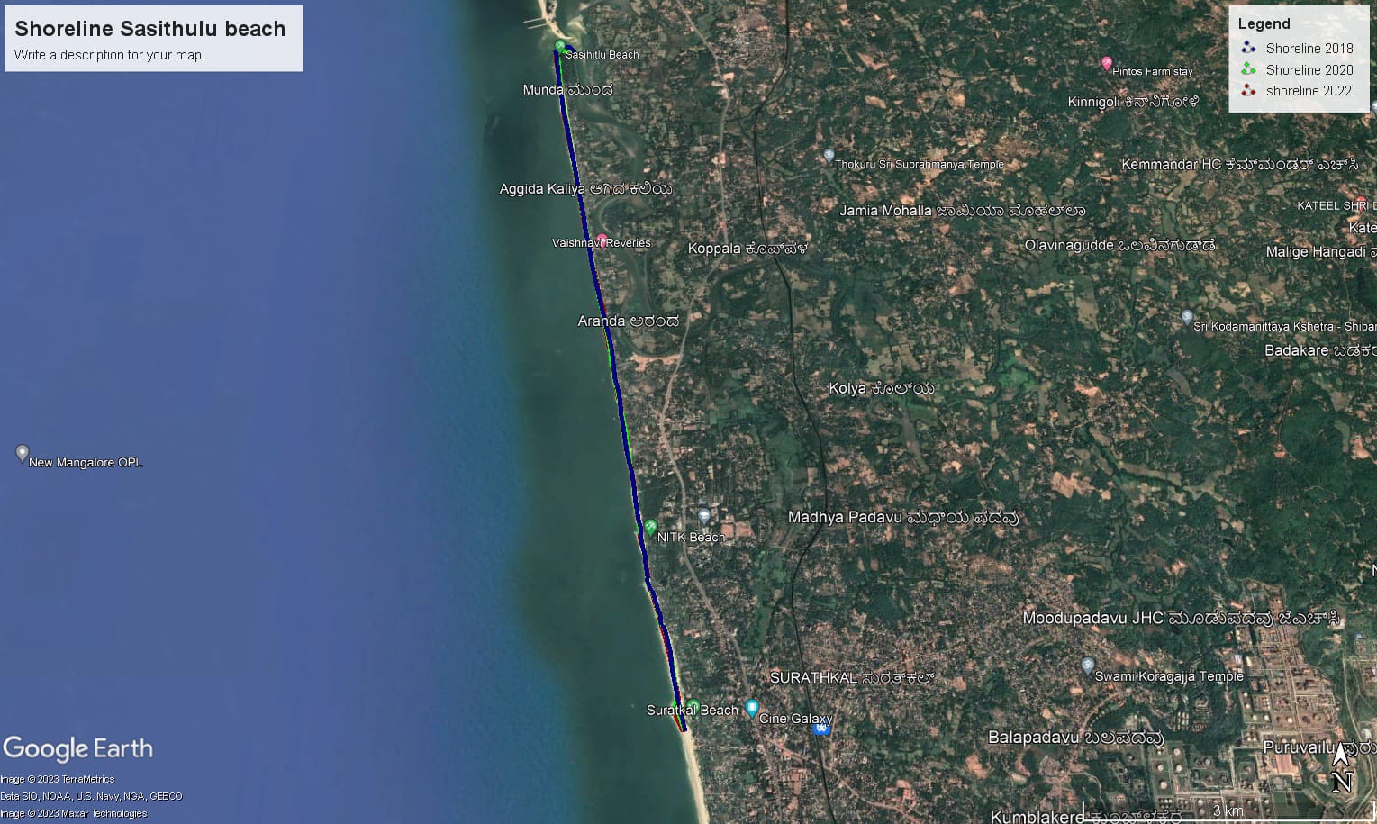
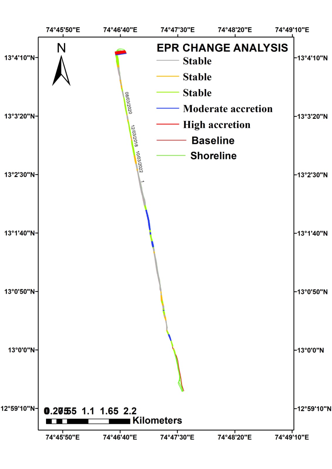
The objective of this study was to analyze the shoreline characteristics and changes of selected beaches using the ArcGIS software and the DSAS (Digital Shoreline Analysis System) extension. The study utilized high-resolution satellite imagery obtained from Google Earth Pro to assess the coastal dynamics and identify patterns of erosion or accretion. Here we have analyzed the beaches from Sasithlu to Surathkal which constitute 9.8km.
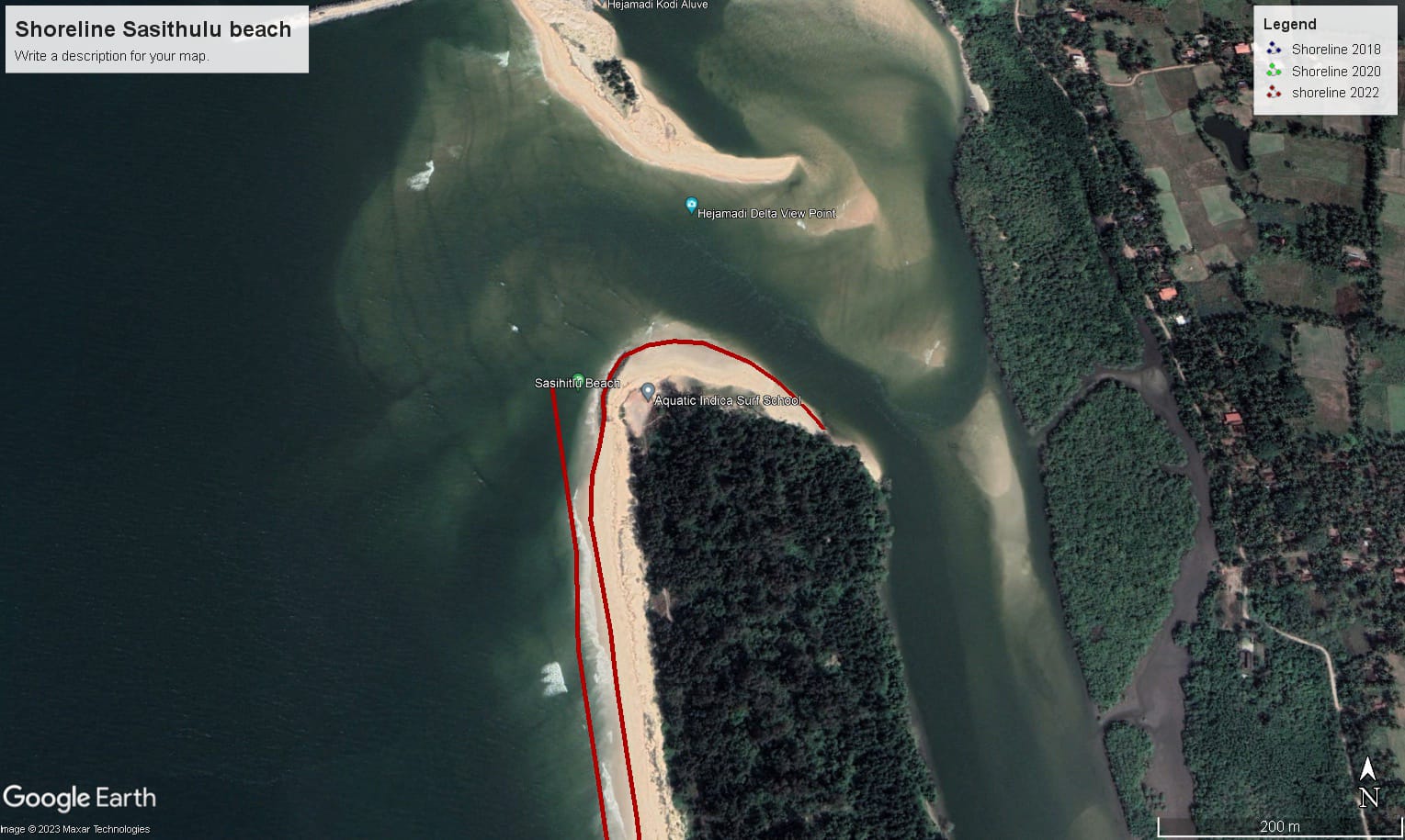
Study area selection
The first step is to select the area which we are going to study and after which do the analysis by plotting the graphs.
Areas are chosen
From Sashithlu beach to Surathkal, which covers almost 9.8ms of the shoreline.
This consists of:
1) Sashithu Beach
2) Mukka Beach
3) NITK beach
4) Surathkal Beach
Data Acquisition
Satellite imagery was obtained from Google Earth Pro, providing detailed imagery of the study area at different time intervals. These images were georeferenced and imported into ArcGIS for further analysis.

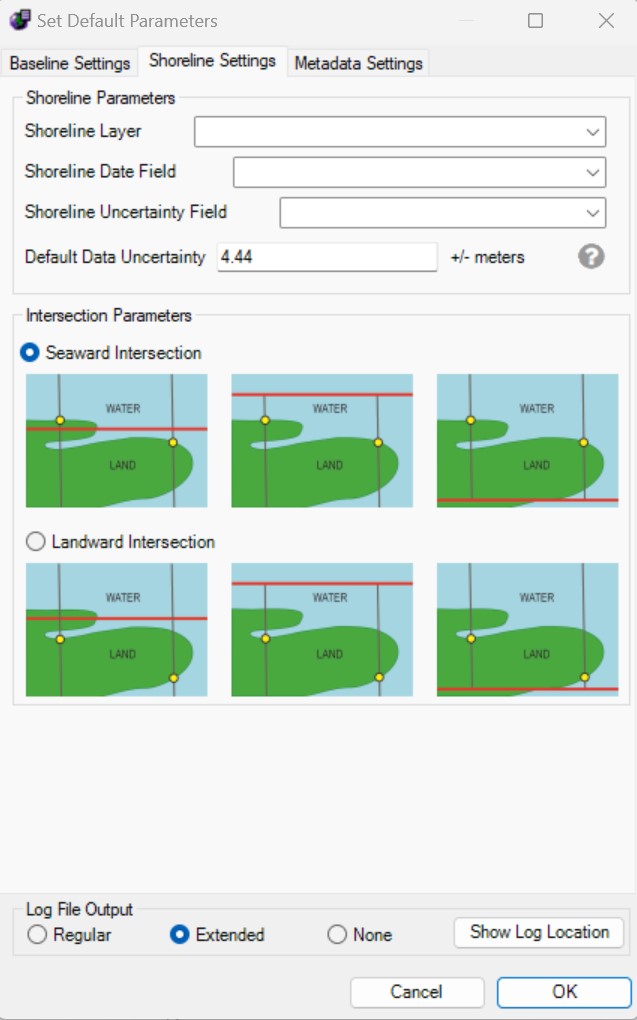
Shoreline Extraction:
The DSAS extension within ArcGIS was utilized to extract the shoreline from the satellite imagery. This process involved manually digitizing the shoreline by identifying distinct features such as the waterline and the land-water interface.
Calculation and plotting:
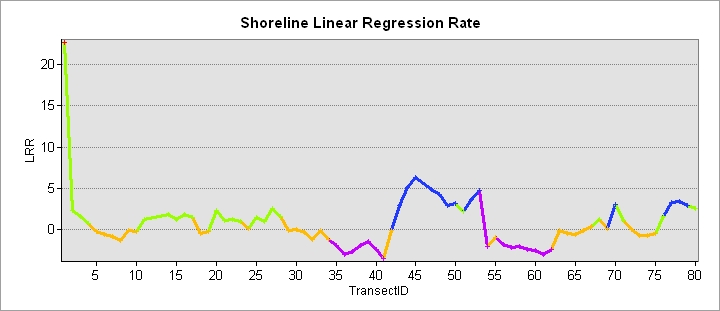
1) Shoreline Linear Regression Rate: The shoreline positions extracted from different time periods were used to calculate the Shoreline Linear Regression Rate (SLRR). SLRR represents the long-term average rate of shoreline change over a specific time interval, providing insight into the overall trend of shoreline advancement or retreat.
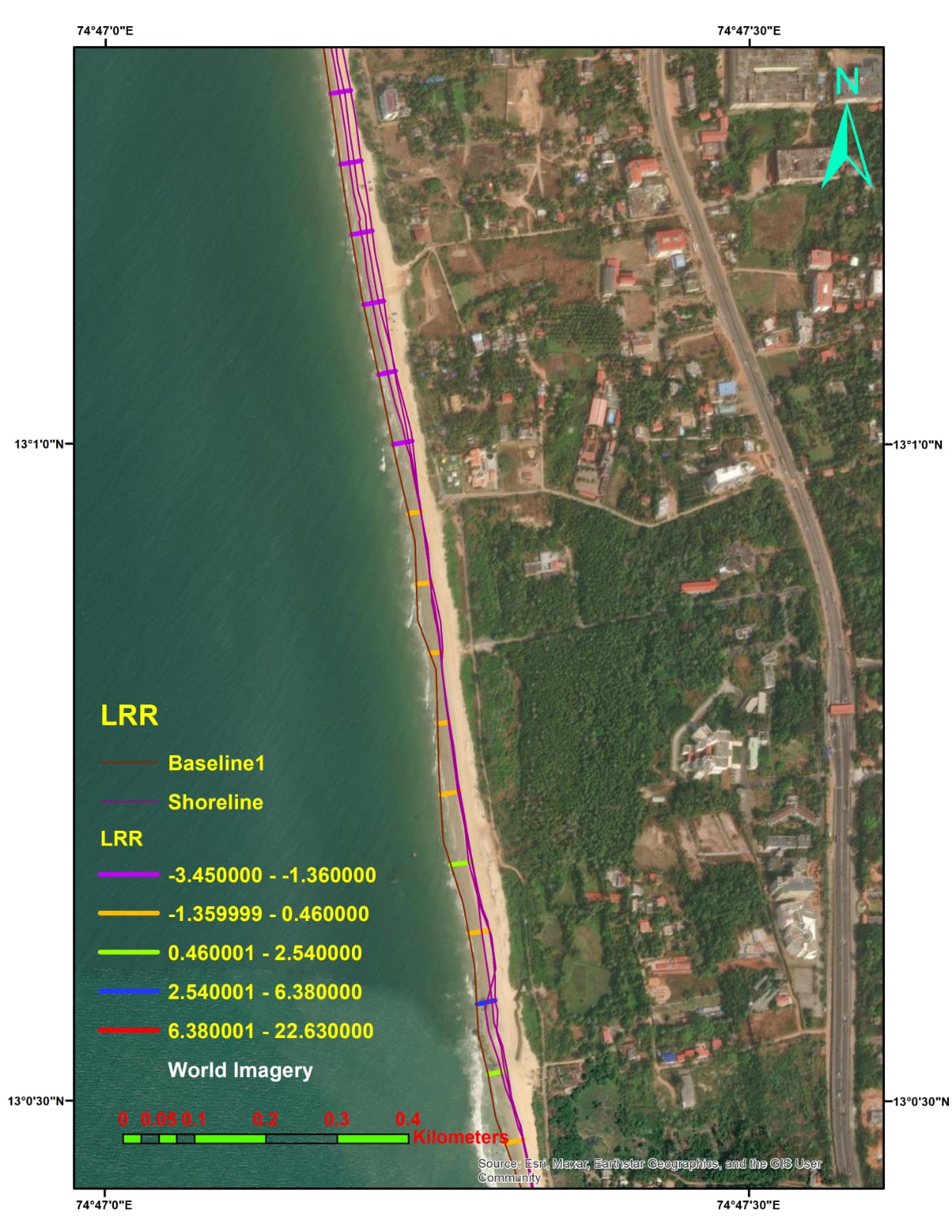
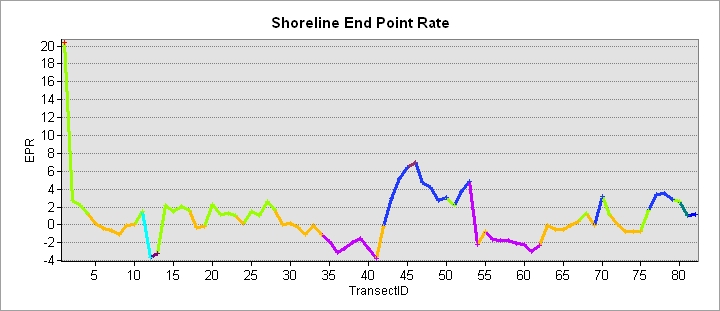
2) End Point Rate (EPR) Calculation: EPR was calculated by measuring the change in shoreline position between two reference points and dividing it by the time interval between the measurements. This provided a quantifiable measurement of the shoreline advancement or retreat.
3) Change Analysis: The SLRR and EPR values were analyzed and plotted over time to visualize shoreline change patterns. The SLRR graph depicted the long-term trend, while the EPR graph showed the temporal variations in shoreline position.
Conclusion:
The study successfully analyzed shoreline characteristics and changes using ArcGIS, the DSAS extension, and Google Earth Pro imagery. The EPR change analysis graph provided a visual representation of shoreline dynamics with the help of the color codings, enabling the identification of erosion-prone or accretion-prone areas. The findings of this study contribute to a better understanding of coastal processes and support informed decision-making in coastal management.
Recommendations
Based on the study’s findings, the following recommendations are proposed:
-
Conduct further investigations to determine the driving factors behind observed shoreline changes.
-
Regularly monitor and update the shoreline data to capture long-term trends and evaluate the effectiveness of coastal management strategies.
-
Integrate the study’s results into coastal planning and management practices to minimize coastal erosion risks and promote sustainable development.
References
Head over to YouTube for playlist GIS
(https://www.youtube.com/playlist?list=PLLy_2iUCG87A2ywI6ZFJPmgq0nGwfBt15)