Mentors
- Jason Krithik Kumar S
- Sidharth Lanka
Mentees
- Chinmaya Sharma
- Sasank Mohan P
- Shama GS
- Vinayak Vatsalya J
- Mohammed Mansoor
Introduction
The objective of this project is to classify given images into their respective classes using Machine Learning.
This is a deep learning project where we aim to implement a CNN pipeline such that we achieve a high accuracy on the task of Object Classification.
We use CNNs as they enable us to exploit the spatial locality of a particular image by enforcing a local connectivity pattern between neurons, while ensuring we minimise the computational cost.
First, we proceed by acquiring a basic understanding of deep learning by implementing MLP and CNN models on the MNIST and Fashion-MNIST datasets. After that we develop a more complex CNN to classify the images of the CIFAR-10 dataset to achieve a high accuracy.
Datasets
We have used two popular datasets namely the Fashion-MNIST and the CIFAR-10 in the course of our project.
Fashion-MNIST
It is a dataset developed by Zalando research, consisting of a training set of 60,000 examples and a** test set** of 10,000 examples. Each example is a grayscale image of 28 pixels in height and width and is associated with a label from 10 classes.

The Fashion-MNIST dataset with label and description of the article
Each pixel has a single pixel value associated with it, the higher numbers meaning darker pixels. This pixel-value is an integer between 0 and 255. The training and test datasets have 785 columns, the first one represents the label and the rest contain pixel values of the associated image. It was developed as a replacement for the MNIST dataset.
We built different models on this dataset and checked for accuracies and losses in a Kaggle Competition.
CIFAR-10
It consists of 60,000 images divided into 10 classes, like aeroplane, deer, frog etc. Each image is a coloured image of 32 pixels in height and width. There are 50,000 training images and 10,000 test images.
A total of 6000 images per class is split into two batches. The testing batch contains 1000 images and the training batch contains 5000 images from each class. The images are randomly distributed and the classes are completely mutually exclusive.
We resorted to a CNN model for this dataset in our project and we validated the model to make predictions more reliable. The dataset is split as 40000 for training, 5000 for validating and 5000 for testing. Here’s a snippet of the CIFAR-10 dataset

Implementation
Kaggle Challenge
The kaggle challenge consisted of training a model on the Fashion-MNIST dataset. We employ PyTorch for the pre-defined functions that speed up the task, matplotlib module to plot and view different images and graphs, NumPy for some basic array operations, and pandas for DataFrame display of data.
Dataloading
This section consists of loading the data from the dataset from torchvision into dataloaders. The data from CSV files are converted to NumPy arrays which are loaded into different loaders. Before loading, we perform normalisation to efficiently scale the data. Then, the data is divided into train and test loaders, and then into batches, which are essentially groups of images. This is done to train the data more efficiently.
Data Visualization
The data is visualized by plotting the data from the .csv file using matplotlib.plt.
Model architecture
We will be using a combination of Convolutional Neural Networks (CNNs) and fully connected layers for the model. Our model is built from several types of layers.
Our model is built from several types of layers:
- Conv2D — performs convolution;
- filters: number of output channels;
- kernel_size: an integer or tuple/list of 2 integers, specifying the width and height of the 2D convolution window;
- padding: Controls the amount of implicit padding on both sides for padding number of points for each dimension;
- max_pool2d : performs 2D max-pooling;
- Linear: Creates fully connected layers;
- Flatten: Flattens the input, does not affect the batch size;
- ReLU: Applies relu activation;
- Dropout: applies dropout;
In this model, one convolutional layer is used with kernel size (3,3) with the number of filters as 9 from 1 (as the images are grayscale). A 2 x 2 max-pooling layer follows this layer. After this, the output obtained is flattened to pass it to the subsequent linear layers. Dropout regularization with p=0.4 is used to avoid overfitting. This is then passed through the first input layer which has the number of inputs equal to the number of outputs from the convolutional and max-pooling layers, and the number of outputs as 64. The ReLU activation function is used after this layer. Then there is another linear layer which has the number of inputs as 64 and outputs as 10, about the 10 classes of classification.
The error function used here is Cross-Entropy Loss, which is defined. The optimizer is defined as Adam, with a learning rate of 0.001.
Model training
The model is passed through a training loop for a given number of epochs. The optimizer.zero_grad() function is used to clear gradients, outputs are found by passing batches of images from the trainloader to the model, the error is calculated using the error function. The backpropagation is done using the optimizer.step() function. Train accuracy is calculated.
Model testing
Model is set for testing using model.eval(). The images from the test loader are looped through and the outputs are found by passing them through the trained model. The test accuracy is calculated.
CIFAR-10
So we’ve seen the theory part, now let’s get to the part where we implement this.
We use Jupyter notebook to implement this code in Python specifically. We use Python as it has a lot of libraries and modules made for Machine learning. We can, of course, try to code every single class and function but this would be time-consuming and we would be just re-inventing the wheel. So we can use the framework PyTorch.
So to begin with we first have to load the data (in this case images from the CIFAR-10 dataset), Python can’t understand images, so we have to convert this into numbers. For this, we use the transforms.Compose() to convert the raw data into tensors. Also, our data is in RGB values in the range (0-255), we normalize this data for improving the model, we can do this by dividing each of the values by 255, so now the range is from (0-1).
We further split the dataset into three portions- train, test, validate using the random_split() function.
- Training Set: Used to train our model, computing loss & adjust weights
- Validation Set: To evaluate the model with hyperparameters & pick the best model during training.
- Test Set: Used to Calculate the final accuracy of our model and to test our model on.
Now we can train using the train entire dataset in one go, but this would be inefficient, therefore we divide it into batches using the DataLoader. Using the dataloader we can load the data in batches. We set shuffle=True for the training dataloader so that the batches generated in each epoch are different, and this randomization helps generalize & speed up the training process.
Each image looks like this :
tensor([[0.5725, 0.5020, 0.4667,  ..., 0.5608, 0.5647, 0.5451],
        [0.5020, 0.4863, 0.4863,  ..., 0.5608, 0.5686, 0.5490],
        [0.4980, 0.5059, 0.5020,  ..., 0.5490, 0.5529, 0.5333],
        ...,
        [0.6314, 0.6353, 0.6549,  ..., 0.6588, 0.6667, 0.6353],
        [0.6431, 0.6431, 0.6392,  ..., 0.6627, 0.6784, 0.6510],
        [0.6431, 0.6431, 0.6353,  ..., 0.6431, 0.6588, 0.6314]])
After loading the data it looks like the array above, but the data is present in batches. The labels are stored correspondingly for each batch as shown below.
tensor([3, 7, 7, 6, 5, 6, 6, 0, 7, 6, 6, 5, 9, 3, 5....])

names = { 0:'Plane' ,1:'Car' ,2:'Bird',3:'Cat' ,4:'Deer',5:'Dog' ,6:'Frog',7:'Horse' ,8:'Boat', 9:'Truck' }
Here, each number corresponds to one of the classes. For example, 1 stands for ‘Car’.
Model
For the model, we will be using a combination of Convolutional Layers and Fully connected layers.
Our model is built from several types of layers:
- Conv2D — performs convolution:
- filters: number of output channels;
- kernel_size: an integer or tuple/list of 2 integers, specifying the width and height of the 2D convolution window;
- padding: Controls the amount of implicit padding on both sides for each dimension’s padding number.
- max_pool2d: performs 2D max pooling.
- Linear: Creates fully connected layers
- Flatten: Flattens the input, does not affect the batch size.
- ReLU: Applies relu activation.
- Dropout: applies dropout.
We will Stack 3 convolutional layers with kernel size (3, 3) with a growing number of filters (16, 32, 64,) with a padding size of 1. We also add a 2x2 pooling layer after every convolutional layer. Now for the fully connected layers, we set the input size accordingly. We will also use the ReLU activation function on the first 3 CNN’s and the next fully connected layer for this model. The final linear layer has 10 outputs corresponding to the 10 classes of images in the dataset.
To reduce overfitting we also added dropouts of probability = 0.25 for the fully connected layers.
We are using hyperparameters, learning rate =0.006 usually set between 0.0001 and 0.1, the number of epochs = 10, optimization function used is SGD, batch size 32 was used. These values can be changed and experimented with to achieve higher accuracy in a shorter time.
Training the model
Now we set the number of epochs to about 20. We can save the best model according to validation. Now for training the model, we loop over the batches of data and calculate the output. Using this output and the actual labels we calculate the loss. Now PyTorch lets us update the weights by optimizer.step().
We can print out the training loss and the validation loss for our reference of how the model is performing after each epoch. Using matplotlib we can plot this as,
Testing our trained model
Evaluating the accuracy vs the number of epochs. Our model reaches an accuracy of around 77-80%


Results
We get a decent accuracy on the CIFAR-10 dataset for models built using just Convolutional Layers and Fully Connected Layers.
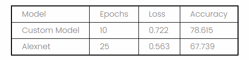
It was seen that the custom model performed much better than the AlexNet architecture model as the latter overfits this small dataset. We could achieve an even higher accuracy if we used transfer learning on the dataset, which we attempt to do in the future.
Conclusion
In this project, we learnt how to implement CNNs from scratch using the PyTorch framework. We explored Kaggle by hosting a competition on it, and building several models that give high accuracy. We also explored AlexNet architecture, as it was among the first CNN architectures which performed extremely well in the ILSVRC Competition. Then, we worked on training a model with good accuracy on CIFAR-10 by implementing the entire pipeline and plotting the results. In the future, we plan to use train the dataset using transfer learning, to achieve a higher accuracy, in an efficient manner.