Project Mentors
- Monal Singh
Project Members
- Aryan Amit Barsainyan
- Rajeev Bhat
- Rushil Raju
Abstract
In recent years there has been increasing research on developing robots containing mechanisms capable of capturing human-link or animal-like behaviors—specifically, the interest in walking bipedal robots emulating human displacement. The interest in diverse fields is continuously emerging, such as replacing humans in hazardous works, rescue operations, military operations, disaster scenarios, or restoration movement in people with disabilities such as dynamically controlled prosthetics. For completion of this project, we will be using MATLAB and Simulink along with SimMechanics. It represents the physical structure, specified through some variables such as mass, geometry, and kinematic relations between its components. It converts this representation into an equivalent mathematical model, which saves time and effort during the development of the mathematical model.
Aim
The project aims to develop a mathematical and mechanical model for a humanoid walking robot by applying kinematics equations and developing the joint models for simulation using Matlab, Simulink, and SimMechanics.
Mechanical Design
The proposed robot is a humanoid walking robot with 6 DOF, including torso, leg, and foot consisting of three revolute joints (hip, knee, ankle) as shown in the figure.
Each rigid body is defined with basic details like dimensions, density, frames, etc., to simulate real-time dynamics. Extending The dimensions are determined using MATLAB variables.
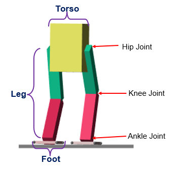
Component 1 - Torso
- Specified dimensions: 0.20 x 0.24 x 0.35m.
- It consists of one frame R with two rigid transformations to which the legs are connected and actuated accordingly.
Component 2 - Leg
- The legs are of dimensions:
- Upper Leg : 0.08 x 0.08 x 0.40m.
- Lower Leg : 0.08 x 0.08 x 0.38m.
- The upper and lower legs have one frame, R, each with two rigid transformations, by which they are connected to the hip, foot, and each other.
- All the connections are made with revolute joints, one degree of freedom joints that allow rotational motion over a common axis.
- The Hip, Knee, and Foot have Revolute Joint.
Component 3 - Foot
- The dimensions : 0.17 x 0.17 x 0.02m.
- It has five frames, namely F1, F2, F3, F4, and A. All the F frames are connected to spherical solids, which incorporate spatial contact force into our model. These spheres have a diameter equal to the height of the foot, which is 0.02 m.
- Frame A is connected to the lower leg.
- The spatial contact forces have stiffness, damping, and friction coefficients that are adjusted accordingly.
Humanoid Motion Pattern Generation
The two essential concepts in humanoid robotics are:
- Centre Of Mass (COM) of the robot where we concentrate all mass of the system and assume where all the mass lies
- Zero Moment Point (ZMP) is where the moment due gravity is exactly canceled out by the moment due to the contact with the ground.
We initially take some approximations that the humanoid bot walks while maintaining a constant height, and the angular momentum around the COM is minimal. This is to model a robot walking on a flat surface. The entire model is approximated as the center of mass. These approximations help us to assume the model is similar to an inverted pendulum model maintained at constant height.
With simple mathematical equations, we can plot the points where the foot shall travel.
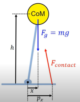
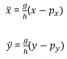
So, from these state dynamic equations, we can generate a center of mass trajectory that is physically consistent. Once the trajectory of the foot is obtained and graphed, inverse kinematics is applied to find the trajectory of the joints and hip (torso).
Inverse Kinematics and its Implementation
Kinematics is the study of motion without considering the cause of the motion, such as forces and torques. Inverse kinematics is the use of kinematic equations to determine the motion of a robot to reach the desired position.
The robot configuration is a list of joint positions within the robot model’s position limits and does not violate any constraints the robot has. Once the robot’s joint angles are calculated using inverse kinematics, a motion profile can be generated using the Jacobian matrix to move the end-effector from the initial to the target pose. The Jacobian matrix helps define a relationship between the robot’s joint parameters and the end-effector velocities.
In Matlab, the inverse kinematics System object creates an inverse kinematic (IK) solver to calculate joint configurations for a desired end-effector pose based on a specified rigid body tree model.
Hence, we were able to generate the desired motion of the joints and commands for the joints so as to make the foot at the correct position to implement walking-like characteristics in the robot.
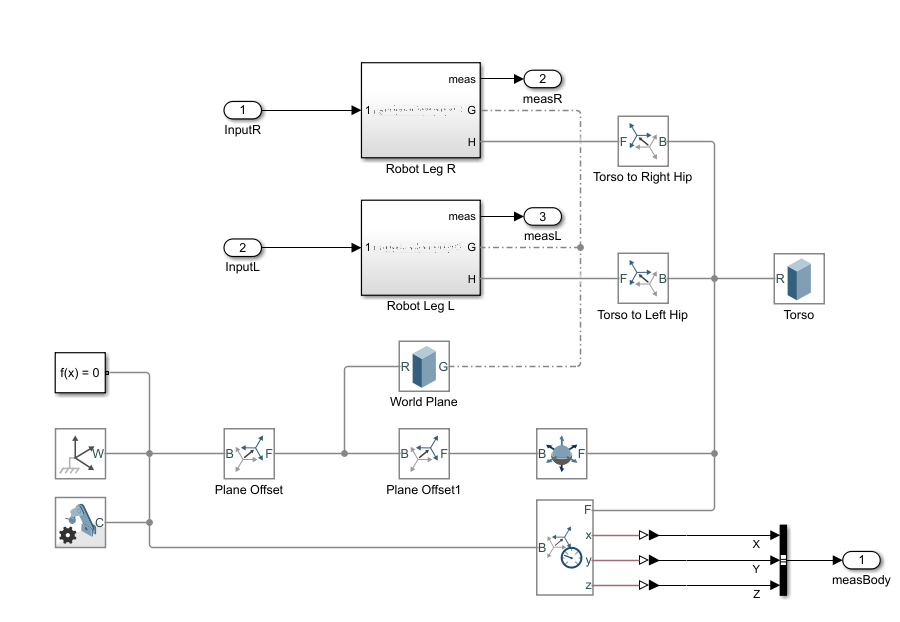
Implementation in Simulink
Inputs and Plant Model
Joint Angles R and Joint Angles L are input blocks corresponding to the variables ‘jAngsR’ and ‘jAngsL‘ respectively. Each store a double matrix containing precise angles to be made by revolute joints after every 0.01 sec to achieve a walking trajectory. These matrices are solutions of the inverse kinematic model based on the trajectory of the robot’s feet to enable it to walk.
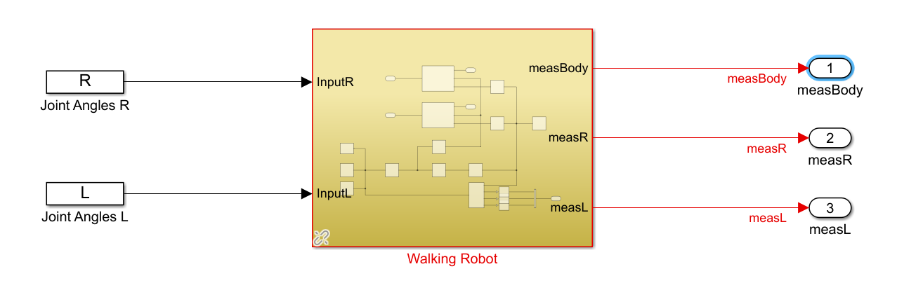
These inputs go into the inputR and InputL ports. From there, the signals are quickly passed into Robot Leg R and Robot Leg L subsystems, respectively. In every system, the signal is transferred to a bus that splits the array of signals into individual signals for every joint present in this subsystem. These signals are passed to motion actuators attached to each of the joints, which ends up in a precise movement of the joints.
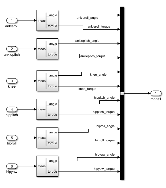
The combined output from each subsystem, Robot Leg R and Robot Leg S, is stored in ‘measR’ and ‘measL,’ respectively. These outputs contain measurements of the angle and torque of each joint in the current configuration.
Mechanical and Simulation Model
The mechanical model of the robot was created using SimScape multibody blocks. We used the solid blocks to develop solid meshes of the world plane (on which the robot walks), torso, upper legs, lower legs, and feet. These were the contact points from the robot body to the world frame and their interaction caused the necessary motions. The revolute joints are used to join the different parts of the robot. A 6-DOF joint was associated with the torso for its free movement across the world frame. This was to ensure that our results were correctly embedded into the controller and model.
Robot Leg Model
Then inputs (joint angles) were connected to the bus, which transferred the input signal to each revolute joint through Simulink-ps converter blocks as shown in the figure.. Then an array is generated from the joint blocks containing information about the current configuration of that joint (torque, speed, and angle). This is to ensure we have entirely controllable as well as visual feedback. This constitutes the forward kinematics of the robot.
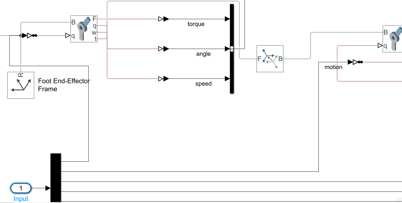 These arrays contain the config info from each joint enter the measurement subsystem, which gives an output ‘meas’ having the current configuration of the entire robot. This essentially contains the mathematical solutions to our project, finally to visualize it, it is sent to the SimScape body. The result is transferred to the inverse kinematic solver to generate joint angles for forward movement at the next instance.
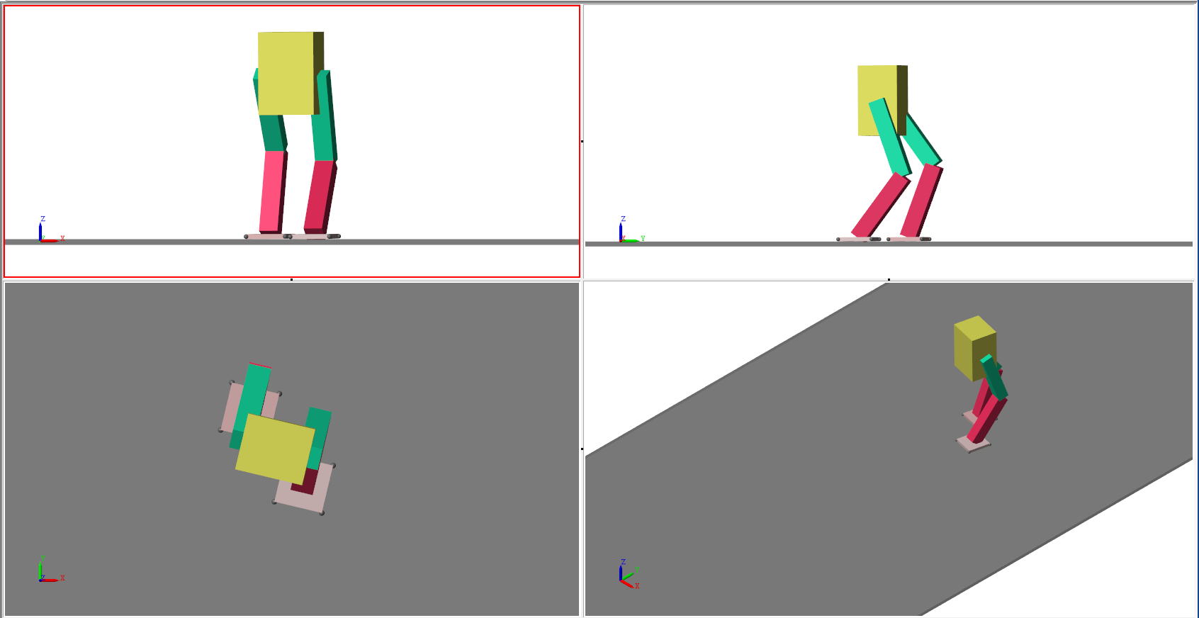
Results
Different perspective views of a still frame of the simulation
Simulation player
The following video shows the final result.
Conclusion
We simulated a model of a bipedal humanoid robot, with a walking trajectory based on the linear inverted pendulum model. The analytical geometry method is adopted to easily obtain the inverse kinematics solution, which has provided the mathematical basis for simulation. The inverse kinematics solver available in MATLAB libraries is used for this purpose. The model is built and simulated using the SimScape multibody app in Simulink. Motion actuation is used to implement the inverse kinematics solution for simulation. The simulation results show that this biped model can walk steadily on flat ground. The optimizations in walking trajectory and use of torque/motor actuators will be a future scope of this project to implement practical simulations applicable in diverse situations.