Mentors
- Rohan Rao
- V Kartikeya
Members
- Dharaneedaran K S
- D R Ashrith
Aim
- To develop a Deep Learning model for segmenting microscopic 2d images of pus cells at various resolutions
- Working with smaller dataset and still achieve high efficiency in model training.
Introduction
Medical image segmentation has an essential role in computer-aided diagnosis systems in different applications.Image segmentation is the procedure of dividing a digital image into a multiple set of pixels. The prior goal of the segmentation is to make things simpler and transform the representation of medical images into a meaningful subject. We tried to tackle this with the help of U-Net architechture. The typical use of convolutional networks is on classification tasks, where the output to an image is a single class label. However, in many visual tasks, especially in biomedical image processing, the desired output should include localization, i.e., a class label is supposed to be assigned to each pixel. Moreover, thousands of training images are usually beyond reach in biomedical tasks. Hence, Ciresan et al.trained a network in a sliding-window setup to predict the class label of each pixel by providing a local region (patch) around that pixel as input. First, this network can localize. Secondly, the training data in terms of patches is much larger than the number of training images. The resulting network won the EM segmentation challenge at ISBI 2012 by a large margin.
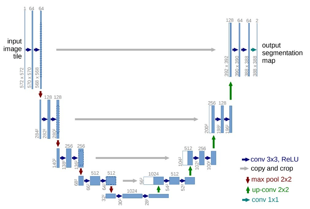
U-Net Architecture
U-Net consists of a contracting path (left side) and an expansive path (right side). The contracting path follows the typical architecture of a convolutional network. It consists of the repeated application of two 3x3 convolutions (unpadded convolutions), each followed by a rectified linear unit (ReLU) and a 2x2 max pooling operation with stride 2 for downsampling. At each downsampling step we double the number of feature channels. Every step in the expansive path consists of an upsampling of the feature map followed by a 2x2 convolution (“up-convolution”) that halves the number of feature channels, a concatenation with the correspondingly cropped feature map from the contracting path, and two 3x3 convolutions, each followed by a ReLU. The cropping is necessary due to the loss of border pixels in every convolution. At the final layer a 1x1 convolution is used to map each 64-component feature vector to the desired number of classes. In total the network has 23 convolutional layers. To allow a seamless tiling of the output segmentation map, it is important to select the input tile size such that all 2x2 max-pooling operations are applied to a layer with an even x- and y-size.
About the DataSet
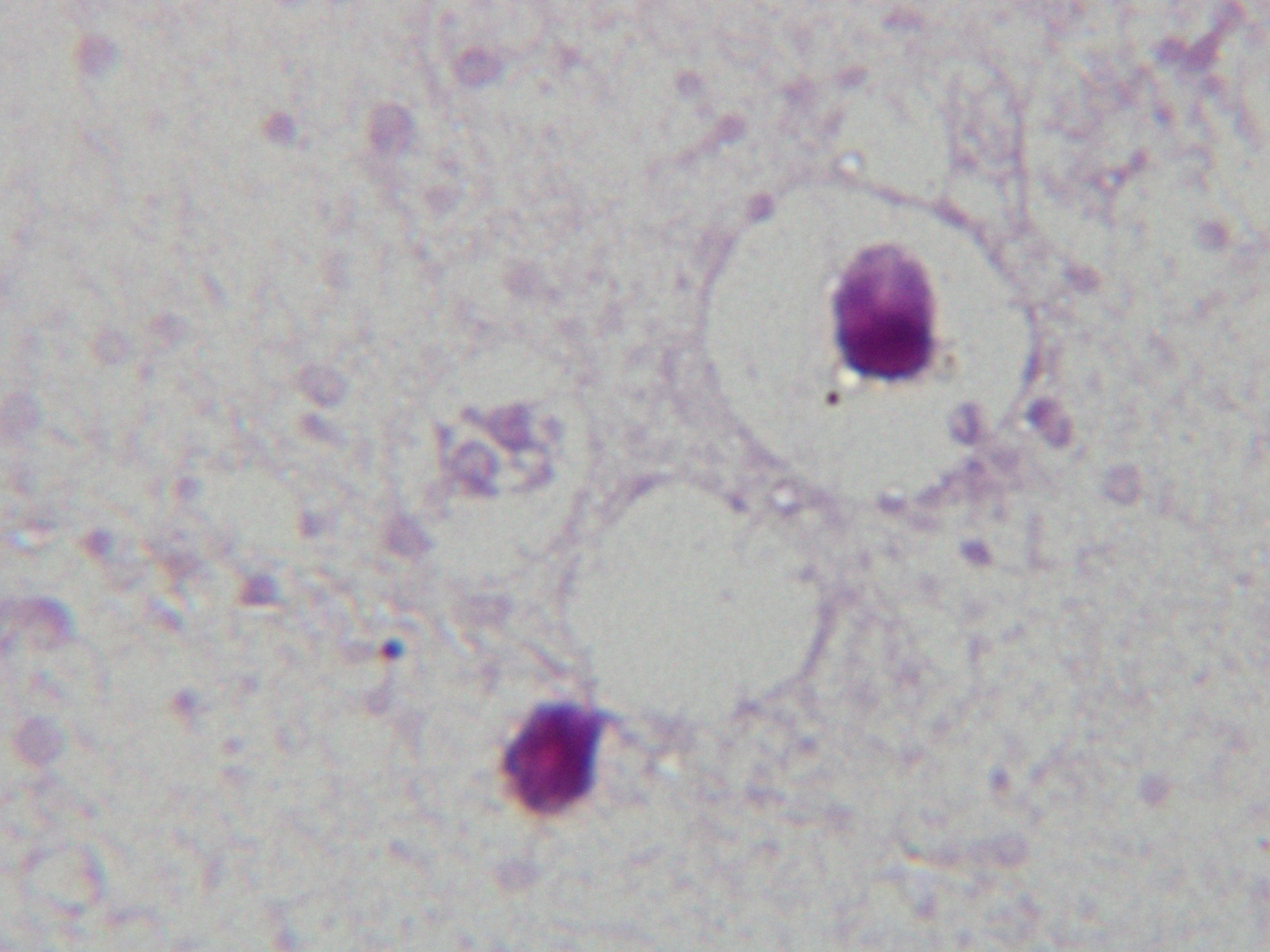
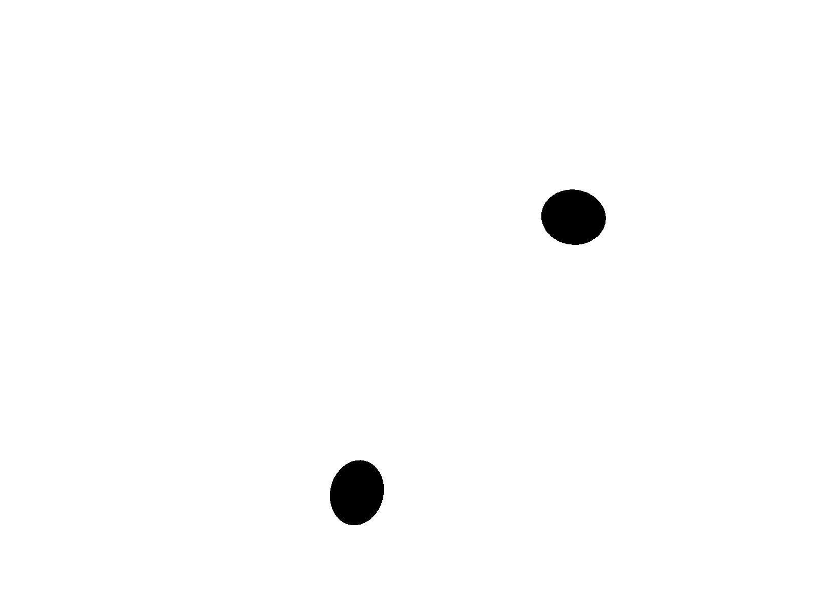
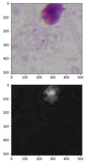
The dataset being used was microscopic images of a resolution of 100X. The input images are of 3 channels, i.e., are color images, with clear distinction of the pus cells being more highlighted by the dye more compared to the rest of the image while the given output, i.e., the masks/labels were of 1 channel, i.e., black and white images, with the segmented pus cell which was seen in black. In contrast, the rest of the image is white. We had a total of 40 image - label pair of images, which was distirbuted as:
- Validation dataset - 5 image pairs
- Train dataset - 30 image pairs
- Test dataset - 5 image pairs
The following are the examlples for the image and its label :
Data Augumentation
Dataset augmentation is the process of applying complex and straightforward transformations to our data set that can help overcome the increasingly large requirements of data sets in a Deep Learning model. For data augmentation, making simple alterations to visual data is popular.
At first, the dataset was divided into three parts with 30,5,5 images as training, validation, and test data set, the function image data generator was used to rotate, flip and resize the corresponding image and its mask for augmenting the data invalidation, test and training data set.
Since our dataset is small, we decided to push it through a data augmentation function called patchifying.
What are patches?
They are the sub boxes of an image at a time for one convolutional layer while it is processed. The function to make patches made overlapping smaller patches of every image and mask in the dataset. Every image was divided into 15 such patches, and this helped us increase the entire dataset by 15 times.
We got a total of 600 image-masks pairs after the entire augmentation was done, with 75 image-masks pairs for testing and validation each and 450 such pairs for training. This helped us increase the dataset significantly.
Training
The augmented data was loaded for training the model and normalized once, and we used the Google colaboratory GPU run-type to train the model. The model was run through multiple iterations of 5 epochs. Trying to get an idea of which parameters (threshold of the sigmoid activation function ) and last activation function to use, we tried to put in various thresholds to correct a few errors, which we were noticing through a few epochs. When the threshold felt adjusted to what felt like the perfect one ( of around -0.2 ), the model was made to train for 40 epochs. The following were the results we received :
- Train accuracy: 95.2%
- train fscore : 0.4366
- train loss: 0.3781
- validation accuracy : 97.8%
- validation fscore : 0.2226
- validation loss : 0.3919
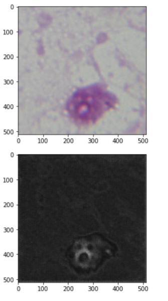
Results
The following are the image and estimated mask by the model:
Conclusion
We were able to train the model with high accuracy using U-Net and were able to train the model with a small dataset.