Combustion Modelling of Sequential Combustion in a Combustor using Adiabatic Flamelet Generated mMnifolds

Mentors

• Erin Sam Joe

Members

• Abhilash Bharadwaj
• A. R. Shriramu
• Erin Sam Joe

Acknowledgements

The members have no acknowledgements to make.

Aim

The aim of the project is to model turbulent, non-premixed combustion processes under realistic conditions.

Introduction

For the detailed design and sizing of a combustion chamber, many OEMs conduct CFD analyses. Due to the size of industrial equipment, it is not possible to conduct direct numerical simulations, requiring appropriate combustion and turbulence models. Single-phase (gaseous) combustion modelling require that the chemical reactions and their kinetics are accounted for, but due to the sherr number of species involved in the combustion of hydrocarbons, solving mass transport equations for all the species would be computational expensive and time-limiting in the design process. Combustion chemistry can be handled through detailed chemistry, reduced chemistry (ARC, CSP, etc. [2]) and manifold-based methods (FGM, SLFM, etc. [3]). Although the latter is not the most precise, it can provide sufficiently precise solutions along with high computational speed.

FGM method has been extended from the basic form to include many different aspects of combustion including heat loss due to radiation, combustion against a reacting surface and spray modelling [4]. Sequential combustion or reheat combustion makes use of the heat and oxidizer present in the exhaust gas of the first combustion stage to initiate and continue combustion in the second combustor. It has been explored within the context of gas turbine combustors as a means of achieving low emissions, enhanced flame stability due to the flame being stabilized by autoignition and flexibility of load and fuel composition [5, 6]. The aim of the present work is to analyse sequential combustion within a combustion chamber.

Materials and Methods

The filtered governing equations for turbulent combustion using FGM - presumed PDF approach can be expressed as follows.

\(\partial_t\tilde \rho + \nabla \cdot (\tilde \rho \tilde u_j) = 0\) \(\partial_t\tilde \rho \tilde u_i + \nabla \cdot (\tilde \rho \tilde u_i \tilde u_j) = - \nabla p + \nabla (2\mu\tilde S_{ij}^D - R_{ij})\) \(\partial_t \tilde \rho \tilde Z + \nabla \cdot (\tilde\rho \tilde u_j \tilde Z) = \nabla (\tilde \rho(\tilde D + D_t) \nabla \tilde Z)\) \(\partial_t \tilde \rho \tilde Y_c + \nabla \cdot (\tilde\rho \tilde u_j \tilde Y_c) = \nabla (\tilde \rho(\tilde D + D_t) \nabla \tilde Y_c) + \bar \omega _{Y_c}\) \(S_{ij} = \frac{1}{2}(\frac{\partial u_i}{\partial x_j} + \frac{\partial u_j}{\partial x_i})\)

where \(S^D_{ij}\) is the deviatoric part of the strain rate tensor \(S_{ij}\) and \(R_{ij}\) is the sub-grid scale (SGS) stress that is provided through the Smagorinsky LES model shown below. \(R_{ij} = \tilde \rho (\tilde{u_i u_j} - \tilde u_i \tilde u_j) = -2 \mu_{SGS} S_{ij}^D + \frac{2}{3}\tilde \rho k \delta_{ij}\)

where \(\mu_{SGS}\) is the SGS viscosity, k is the SGS kinetic energy defined by, \(\tilde \rho k = \frac{1}{2}\tau_{kk} = \frac{1}{2}\tilde \rho(\tilde{u_k u_k} - \tilde u_k \tilde u_k)\)

The SGS viscosity is closed by the Smagorinsky model that models the eddy viscosity in equation (8). \(C_s\) is the Smagorinsky constant and \(\Delta\) is the filter width, which in the case of implicit LES filtering is directly related to the mesh size. \(\mu_{SGS} = C_s \Delta^2|\bar S| = C_s \Delta^2\sqrt{2 \bar S_{ij} \bar S_{ij}}\)

\(k_{SGS}\) is obtained from the balance equation to simulate the behavior of subgrid kinetic energy as shown in equation (9). The constants \(C_*\) and \(D\) are positive coefficients representing the kinetic energy dissipation and diffusion respectively. \(\partial_tk_{SGS} + u_j\nabla k_{SGS} = -\tau_{ij}\bar S_{ij} - \frac{C_*}{\Delta}k_{SGS}^{3/2} + \nabla (D\Delta \sqrt{k_{SGS}} \nabla k_{SGS}) + \mu \nabla^2k_{SGS}\) The scalar transport equations (3) and (4) are the transport equations for the mean mixture fraction and the mean unscaled progress variable, which serve as the control variables. Further explanation of these terms can be found in the next subsection.

Flamelet Generated Manifolds

From time scale analyses of a number of combustion systems, it is possible that the reaction path in composition space is embedded in a low-dimensional manifold, which can be described by a small number of control variables [7]. Thus it is possible to map a single state in a combustion system to a manifold given by its control variables — a simple selection of control variables that does not account for heat losses (convection at walls, by radiation, etc.) would be the mixture fraction, \(Z\) and the progress variable, \(Y_c\) . Physically, the mixture fraction represents a mapping between the composition at pure oxidizer and the composition at pure fuel and the progress variable physically represents a mapping between the completely unburnt and completely burnt state at that point within the system.

The manifold solution is obtained from solving the flamelet equations of a counterflow diffusion flame, equations (10) through (13) . Cantera is used to solve these equations and takes into account the detailed chemical kinetics. The GRI Mech 3.0 mechanism that is capable of the representation of natural gas flames and ignition.

\(\frac{\partial \rho u}{\partial z} + 2 \rho V = 0\) \(\rho u \frac{\partial V}{\partial z} + \rho V^2 = -\Lambda + \frac{\partial}{\partial z}(\mu \frac{\partial V}{\partial z})\) \(\rho c_pu\frac{\partial T}{\partial z} = \frac{\partial}{\partial z}(\lambda\frac{\partial T}{\partial z}) - \sum_k j_k c_{p,k}\frac{\partial T}{\partial z} - \sum_k h_k W_k\dot \omega_k\) \(\rho u \frac{\partial Y_k}{\partial z} = -\frac{\partial j_k}{\partial z} + W_k\dot \omega_k\)

The mixture fraction is calculated using Bilger’s formula [24], \(Z = \frac{b - b_o}{b_f - b_o}\)

where \(b = 2 \frac{Y_C}{W_C} + 0.5\frac{Y_H}{W_H} - \frac{Y_O}{W_O}\) subscripts correspond to the elements C, H and O. The subscripts o and f correspond to the oxidizer and the fuel stream. In the present study, the progress variable is defined as, \(Y_c = 4\frac{Y_{H_2O}}{W_{H_2O}} + 2\frac{Y_{CO_2}}{W_{CO_2}} + 0.5\frac{Y_{H_2}}{W_{H_2}} + \frac{Y_{CO}}{W_{CO}}\)

The scaled progress variable is defined as, \(C = \frac{Y_c - Y_c^u}{Y_c^b - Y_c^u}\). The superscripts u and b represent unburnt and burnt states. The solution of manifold equations (10) through (13) provide solutions for a flamelet, which contains the required data (scalars which shall be looked up during run time), \(Y_k\), \(\bar \rho\), \(\tilde T\), \(\alpha\), \(\mu\), \(\bar \omega_{Y_c}\), etc. at different values of strain rate, \(\chi\). In the present work, the strain rate is modified by changing the inlet velocity [9]. The required data is then stored in tables to be looked up by \(\tilde Z\), \(\tilde Z''^2\), \(\tilde C\) and \(\tilde C''^2\), after convoluting with the PDFs which is described in the next subsection.

Table Generation

iTurbulence-flame interasctions, i.e., subgrid chemistry effects, for LES of turbulent combustion can be handled in two ways — presumed PDF approach [10,11] or a thickened flame approach [12, 13]. The former is selected in the present work and extends the storage of data from 2D (in terms of \(Z\) and \(C\)) to storage in 4D (in terms of \(\tilde Z\), \(\tilde Z''^2\)$, \(\tilde C\) and \(\tilde C''^2\)). The favre-averaged / filtered scalars are calculated as, \(\tilde \phi = \int \int \phi(Z,C)\tilde P(Z,C|...)dZ dC = \int \int \phi(Z,C)\tilde P(C|...)\tilde P(Z|...)dZ dC\) where \(\tilde P( )\) is the \(\beta\)-function, which is a good representation of the PDF of mixture fraction and the scaled progress variable.

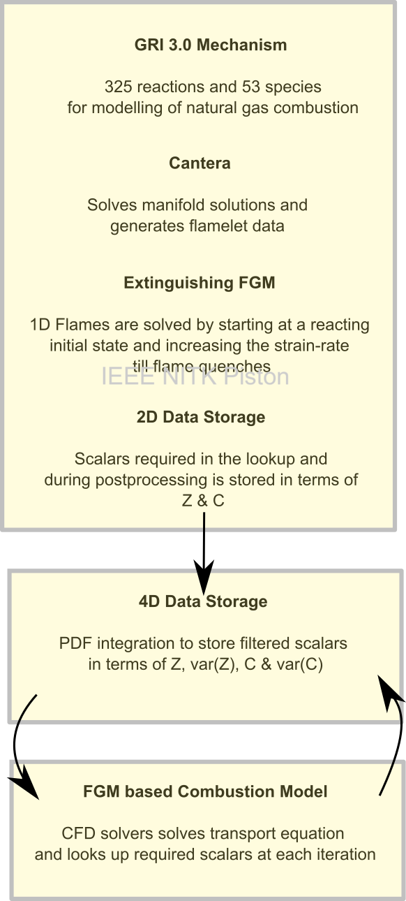
The CFD solver, having solved the transport equations (3) and (4), can calculate the variance of Z and C, and then proceed to look up the values for the filtered scalars during run time. A pressure-based CFD solver, using finite-volume discretization, was developed within the framework of OpenFOAM, along with a new combustion model that adds the source term on the RHS of equation (3), and the lookup-procedure is handled through OpenFOAM’s class IOdictionary. Python scripts are used for table generation from the manifold solutions obtained using Cantera. Figure 1 provides an overview of the workflow from flamelet generation, tabulation, to table-lookup in the CFD solver.

Computational Model

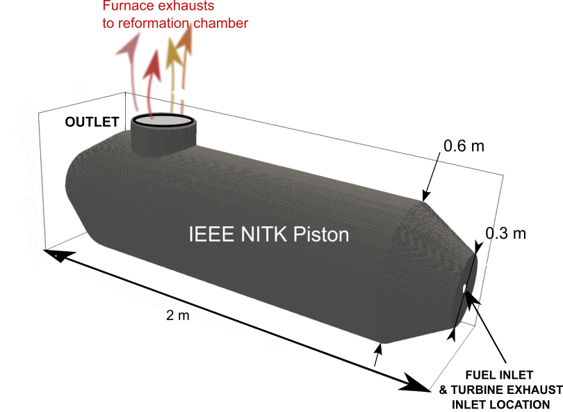
The schematic diagram of the combustor is shown in Figure 2. The combustor is located downstream of a commercial gas turbine (GT). The combustor is fired through the sequential combustion of natural gas and the excess oxygen in the GT exhaust flue gas. The fuel inlet is located at center of the annotated face with a diameter of 20 mm and the turbine exhaust (oxidizer) inlet is modelled as concentric to the fuel inlet, with an outer diameter of 100 mm. The mean fuel stream inlet velocity is 15 m/s and the mean oxidizer stream inlet velocity is 30 m/s. The entire flow field within the furnace is initially quiescent. The walls of the furnace are considered to be adiabatic, and zero-gradient boundary conditions are applied during the solution of equations (1) through (4). Since the generated mesh has \(y^* > 1\) , wall functions are used to model the interaction of kinetic energy and turbulent eddy dissipation rate at the walls. Navier-Stokes characteristic boundary conditions (NSBC) were imposed on the inlet and the outlet [14]. The geometry shown in Figure 2 was modelled in GMSH and meshed using SnappyHexMesh. The mesh size was selected to be sufficiently fine to achieve the condition that at most 20% of the kinetic energy is modelled for good accuracy in LES [15].

Validation

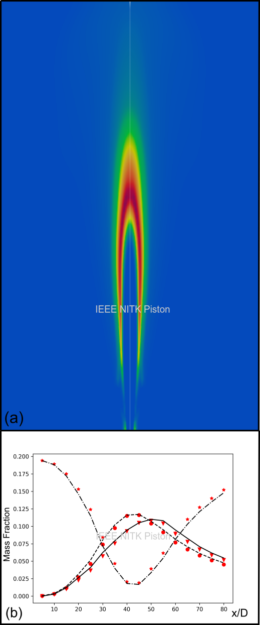
The developed solver, along with the tabulated data, is validated against the time-averaged data for the Sandia-D flame in Figure 3. The solver, having shown good agreement with the experimental data of the Sandia-D flame, gives us a degree of confidence in the analyses done using it.

Results and Discussion

The transient (instantaneous field) results presented within this section are that of a state within the SMR furnace when the time-averaged results cease to show a distinguishable difference.

Flow Features

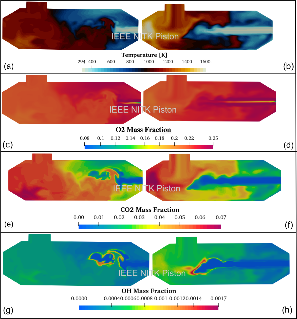
Figure 5 (c) and (d) show an instant of the velocity field within the combustor. The flow in both cases are filled with eddies that provide mixing between the fuel and oxidizer streams, which aids in combustion of the fuel mixture earlier along the length of the furnace from the fuel inlet. The magnitude of velocity is larger at the inlets and increases at the outlet, the latter which can be attributed to a decrease in area and increase in pressure by formation of combustion products which aids in driving the flow. In figure 5 (d), the velocity magnitude approaches and gets close to the speed of sound of the mixture, the design should take into account that no shocks form in the outlet of the furnace which would result in the flow getting choked. This phenomena is not studied in detail in the present work, but it would place a limit on how fast combustor exhaust gases can be evacuated and may result in a dangerous pressure build up within the chamber.

Figure 4 (a) and (b) provide level-set contour of the instantaneous temperature field within the combustor for case 1 and 2 respectively. Since case 2 has a higher equivalence ratio, the flame is held further down in the chamber and provides a higher temperature, as compared to case 1. This may be detrimental to the service life of the furnace that may face creep or thermal fatiguing, with the highest temperature located at the end face. Figure 5 (c), (d), (e), (f), (g) and (h) show transient field distributions of mass fractions of species \(\textrm O_2, \textrm{CO}_2\) and \(\textrm{OH}\). Figure 5 (c) and (d) show that not all the oxygen provided by the oxidizer gets consumed. This can be overcome with a well-designed nozzle to enable a higher degree of mixing or increasing the fuel flow rate. Figure 5 (g) and (h) show the locations of high concentrations of the intermediate combustion species, \(OH\) , where the flame edge fronts are located. Case 2, for the given slice, shows a far deeper penetration and implies that a majority of the combustion takes place almost directly under the chamber outlet. Case 1, shows itself having the flame being held nearer to the inlets and highly affected by the turbulent flow field.

Flame Features and Vortex-Flame Interaction

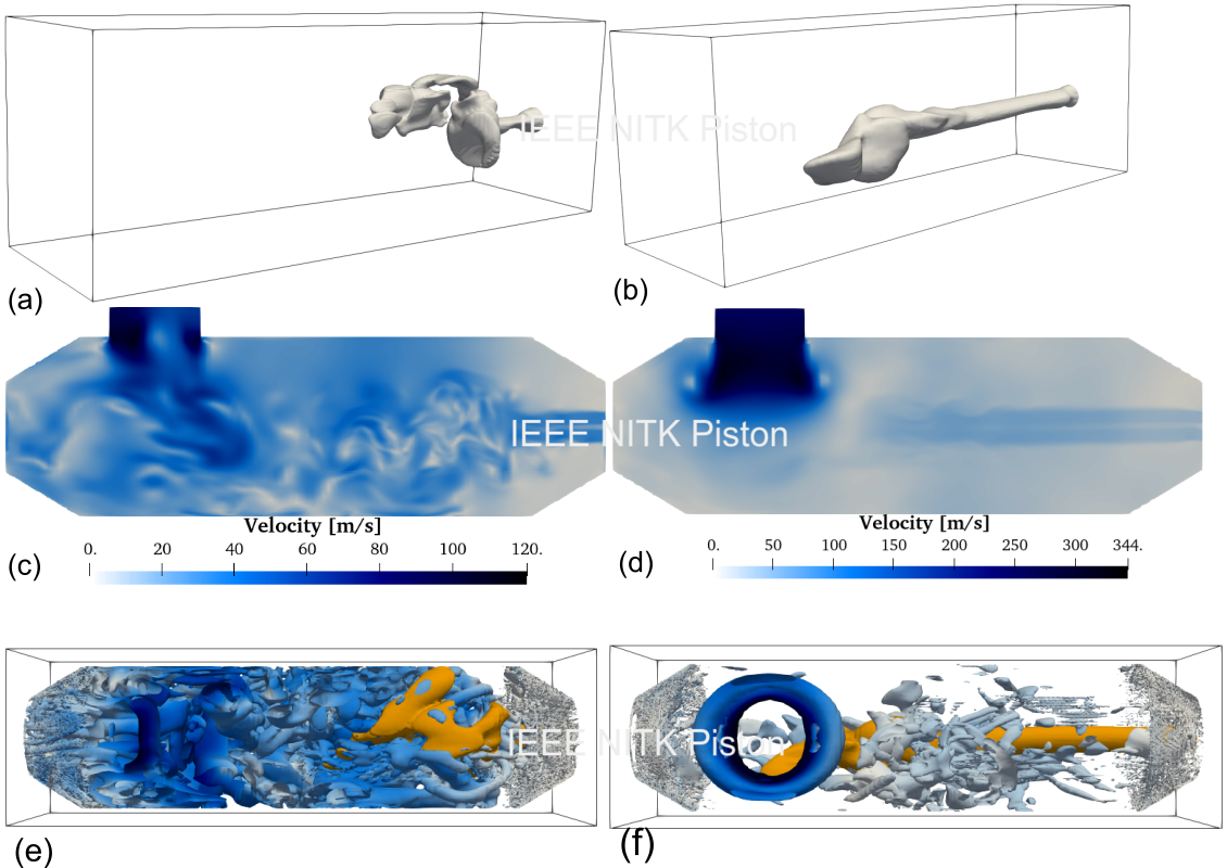
Figure 5 (a) and (b) identifies the flame surface by using an iso-surface scaled progress variable value of 0.9. The length of the unaffected jet from the inlets is much shorter in case 1, than in case 2. Case 1 shows no break up of the fuel stream, but is visible in case 2. The high degree of liftoff in case 2 is rather dangerous, raising concerns of flame stability. The local flow speed should be decreased in comparison to the local laminar flame speed by decreasing the mean fuel inlet velocity, but with maintaining the criteria that local laminar flame speed less than the local flow speed to avoid the possibility of flashback [16, 17]. Figure 5 (e) and (f) show iso-surfaces of Q-criterion that aid in the identification of vortical structures. Case 1 shows a far more turbulent flow field that may have allowed for the faster mixing of the fuel and oxidizer streams and shorter flame brush. Figure 5 (f) shows a toroidal vortex (also found in time-averaged results) at the outlet. Such a flow structure can lead to erosion of the combustor refractory, being contacted by highly convective flows, complex chemical phenomena and high thermal stresses [18].

Conclusion

Sequential combustion within a combustion chamber was modelled using adiabatic Flamelet Generated Manifolds (FGM) for combustion modelling. A pressure-based solver, discretized using the finite-volume method, was developed for this purpose within the framework of OpenFOAM and was used to analyse flow features, flame structure and vortex-flame interaction. The species mass fraction, temperature profiles and velocity field were analysed to understand flow structures. The flame structure and vortex-flame interaction was studied using Q-criterion iso-surfaces and observing the flamesheet from an iso-surface of the scaled progress variable. The first case studied showed a more stable flame, although with a low temperature at the outlet and wasting quite a bit of oxygen. The second case studied showed a potentially unstable and unsafe flame, that may result in the damage of furnace if not redesigned and danger to operators.

References

1. Herraiz,Laura;Lucquiaud, Mathieu;Chalmers, Hannah; Gibbins, Jon (2020).Sequential Combustion in Steam Methane Reformers for Hydrogen and Power Production With CCUS in Decarbonized Industrial Clusters. Frontiers in Energy Research, 8(), 180–.
2. Malpica Galassi, Riccardo; Valorani, Mauro; Najm, Habib N.; Safta, Cosmin; Khalil, Mohammad; Ciottoli, Pietro P. (2017). Chemical model reduction under uncertainty. Combustion and Flame, 179(), 242–252.
3. H Müller, F Ferraro, M Pfitzner, (2013). Implementation of a Steady Laminar Flamelet Model for nonpremixed combustion in LES and RANS simulations. 8th International OpenFOAM Workshop.
4. Maghbouli, Amin; Akkurt, Berşan; Lucchini, Tommaso; D’Errico, Gianluca; Deen, Niels G.; Somers, Bart (2018). Modelling compression ignition engines by incorporation of the flamelet generated manifolds combustion closure. Combustion Theory and Modelling, (), 1–25.
5. Schulz, Oliver; Noiray, Nicolas (2019). Combustion regimes in sequential combustors: Flame propagation and autoignition at elevated temperature and pressure. Combustion and Flame, 205(), 253–268.
6. Güthe, Felix; Hellat, Jaan; Flohr, Peter (2009). The Reheat Concept: The Proven Pathway to Ultralow Emissions and High Efficiency and Flexibility. Journal of Engineering for Gas Turbines and Power, 131(2), 021503–.
7. van Oijen, J.A.; Donini, A.; Bastiaans, R.J.M.; ten Thije Boonkkamp, J.H.M.; de Goey, L.P.H. (2016). State-of-the-art in premixed combustion modeling using flamelet generated manifolds. Progress in Energy and Combustion Science, 57(), 30–74.
8. Bilger, R.W., Starner, S.H., Kee, R.J. On reduced mechanisms for methane/air combustion in nonpremixed flames. Combustion and Flame, 80 (2), pp. 135-149,1990.
9. Fiala, Thomas; Sattelmayer, Thomas (2014). Nonpremixed Counterflow Flames: Scaling Rules for Batch Simulations. Journal of Combustion, 2014(), 1–7.
10. Han, Chao; Wang, Haifeng (2017). A comparison of different approaches to integrate flamelet tables with presumed-shape PDF in flamelet models for turbulent flames. Combustion Theory and Modelling, (), 1–27.
11. F. Liu; H. Guo; G.J. Smallwood; Ö.L. Gülder; M.D. Matovic (2002). A robust and accurate algorithm of the β-pdf integration and its application to turbulent methane–air diffusion combustion in a gas turbine combustor simulator. , 41(8), 763–772.
12. Colin, O.; Ducros, F.; Veynante, D.; Poinsot, T. (2000). A thickened flame model for large eddy simulations of turbulent premixed combustion. Physics of Fluids, 12(7), 1843–.
13. P.J O’Rourke; F.V Bracco (1979). Two scaling transformations for the numerical computation of multidimensional unsteady laminar flames. , 33(2), 185–203.
14. T.J Poinsot; S.K Lelef (1992). Boundary conditions for direct simulations of compressible viscous flows. , 101(1), 104–129.
15. Stephen B. Pope, Turbulent Flows, Cambridge University Press, 2000.
16. Gollahalli, S.R.; Savaş, Ö.; Huang, R.F.; Rodriquez Azara, J.L. (1988-01-01). “Structure of attached and lifted gas jet flames in hysteresis region”. Symposium (International) on Combustion . 21 (1): 1463–1471.
17. Demare, David; Baillot, Françoise (2001-05-30). “The role of secondary instabilities in the stabilization of a nonpremixed lifted jet flame”. Physics of Fluids
18. Guzmán, A.M.; Martínez, D.I.; González, R. (2014). Corrosion–erosion wear of refractory bricks in glass furnaces. Engineering Failure Analysis, 46(), 188–195.