A Convolutional Neural Network.
A Convolutional Neural Network and 90 minutes of training
Clearly, the hard part wasn’t the training or the model but to get the training set.
But what is the data? and where did we get it form?
On December 14, 2017 NASA announced the discovery of an eigth planet in the Kepler-90 system. Kepler-90 is a Sun-like star 2545 light-years from Earth. The discovery was made using Artificial Intelligence.
Where did the data come from?
NASA has this huge camera up in space that has been sending us videos of stars of interest every 29.4 minutes. That’s an oversimplification of what the Kepler Space Telescope does, but it’s enough for the purpose and essence of this article. Kepler’s 94.6 megapixel[1] camera has a fixed field of view, which means it’s been looking at the same spot in the sky since it launched in 2009.
That’s a lot of data.
What is the data?
To understand the data, we need to first understand how NASA detect planets. Planets don’t emit light. So how does Kepler even see planets that are lightyears away? Planets don’t emit light… but Stars do. Kepler measures the brightness of stars over several years and since planets orbit around stars, they must cross the line of sight between kepler and the star periodically.

So, Kepler puts up a nice brightness vs time graph and sends it back to us every 29 minutes. A periodic dip in the graph implies that there must be a planet. NASA classified periodic dips that may be consistent with transiting planets as Threshold Crossing Events (TCE). The Kepler team initially heterogenously put together TCEs by hand, but later on they designed an Auto Vetter that automatically eliminates uninteresting candidates.
And this gives the raw unprocessed dataset: The Autovetter Planet Candidate Catalogue hosted at the NASA Exoplanet Archive. The light curves that were used to find the new planets are from the Mikulski Archive for Space Telescopes. Each light curve in this dataset consists of integrated flux (brightness) measurements spaced at 29.4 minute intervals for upto 4 years[2].
Processing the dataset
The researchers at NASA then followed this up with flattening the light curve by fitting a basis spline (removes the low frequency variability) and then dividing it by the best-fit spline (connect the dots and smoothen them).
They had to then fold (to make it event centered[3]) and bin the flattened curve to produce a 1D vector.
Binning and folding are two methods of making trends in messy data more apparent.
Folding is useful when a source has periodic variability; the data is plotted in terms of phase, such that all the data are plotted together as a single period, in order to see what the repeated pattern of variability is.
Folding is basically splitting the graph into blocks and then overlapping all the blocks on top of one another. This way we can notice repeated patterns more easily.
Random variations from this pattern can be reduced by binning the data in time, which involves splitting the phase range into steps (bins) in which all the data are averaged, using a weighted mean.
Even if we do fold the graph, it’s still really messy since there may be random variations in the data. Binning can be thought as averaging the data out at a folded point in time to give 1 point.
| Original Light Curve | Folded Curve | Binned Curve |
|---|---|---|
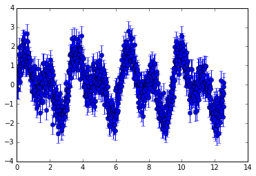 |
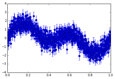 |
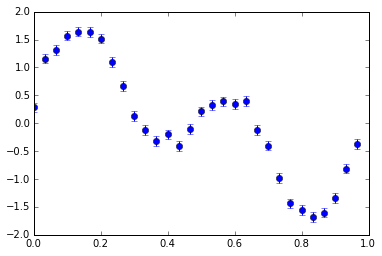 |
The problem with binning the TCE dataset is that all the periods in our light curves are of different lengths. Different planets have different orbital lengths, different orbital periods and different distances from Earth. Hence, different periods of transits. So, how did they bin these light curves to act as inputs?
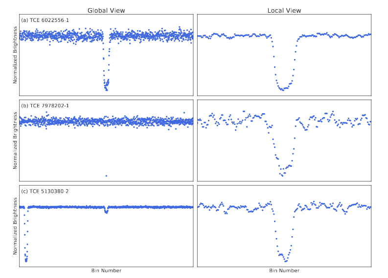
They generated two separate views of the same light curve:
-
A global view which was generated by binning by a fraction of the TCE period. These views, the global views of the light curves, were all binned to the same length, and each view represents the same number of points, on average, across all light curves.
-
A local view which was generated by binning by a fraction of the TCE duration. This results in a zoomed in view of the TCEs. It treats short and long TCEs equally and so might miss out on some information. It looks at only a part of the curve.
The dataset is now ready.
The researchers then passed these views as inputs into the their multilayered convolutional network and trained.
Resources
Although this post is not going to divulge into the details of the neural network, you can check it out on their research paper: Identifying Exoplanets with Deep learning.
If you want to know more about binning, folding and how to apply them with numpy, go here.
[1] Kepler only sends back about 5% of the 94.6MP based on our Stars of Interest
[2] Roughly 70000 points
[3] There are 4 years of data and planets don’t cross all the time. So, we need to remove the parts where they aren’t crossing.
