Introduction to Reinforcement Learning
Reinforcement learning(RL) is a branch of machine learning which draws from the way humans learn to do tasks. For anyone unfamiliar with Pavlov, he is a physicist popularly known for his work in conditioned response. He trained a dog such that every time he rang a bell, he would immediately give the dog food. The dog soon learned to salivate at the sound of the bell. The same foundation to Jim’s mint prank in The Office for those who get the reference xD.
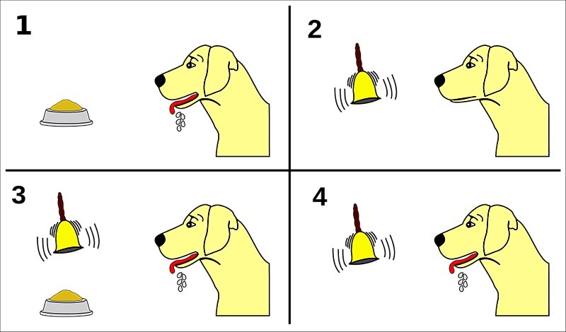
Reinforcement learning (or RL) takes Pavlov’s experiment one step further. Suppose the new experiment was that when Pavlov rang each bell out of a set of them, the dog would have to perform some corresponding trick to receive his treat. The dog, through trial and error, would eventually observe and learn the correct action to take for each bell to get as many treats as he can. This is essentially how dog-training and, you guessed it, RL in its basic form works!
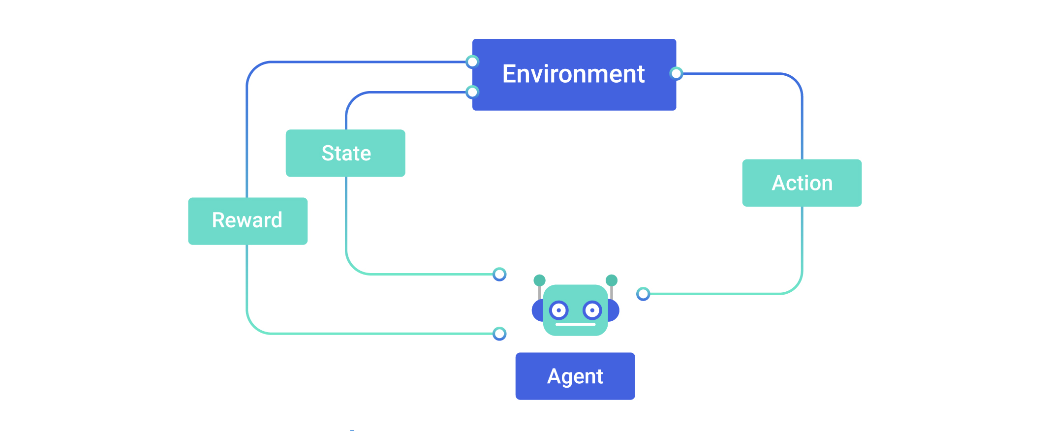
For a quick insight into the technical basics of RL, it is a setup where an agent (our dog) takes an action in some environment and then receives observations (the different ringing bells) and reward (yummy treats) from that environment. The environment consists of states (in this case, what bell is ringing), and in each state, the agent takes an action to get to another state. While the next state and reward received are out of the agent’s control or full prior knowledge, what it can do is learn from those findings to take better actions. The fundamental objective is to maximize the cumulative expected reward, also called expected return. Depending on the factor γ, also called the discounting factor, the amount of importance given to future rewards may be reduced. γ decides how short-sighted or far-sighted the agent is, i.e: how much it prioritizes reward it receives in the near future compared to what it would receive later.
What is referred to as the agent’s policy can be thought of as a strategy while playing a game. More formally, it’s a function that maps a state to an action or a distribution over actions. We also define an action-value function, Q that gives us a measure of how good it is to take a particular action in each state, or to know how favorable each action is in a state of the game. There is also a state-value function which tells you how good it is to be in each state. It is the expected reward that is obtained by following a given policy, starting from that state.
All this sounds very similar to a human playing a game, and you’re right, it really is. The usual concept of points conveniently plays the role of reward. So, let’s understand it better by playing the casino card game of blackjack.
Blackjack rules
Here are the basic rules
Here all face cards have the value of 10. The game begins with two cards dealt to both dealer and player. One of the dealer’s cards is face up and the other is face down. If the player has 21 immediately (an ace and a 10-card), he wins unless the dealer also has the same, in which case the game is a draw. If the player does not have 21, then he can request additional cards, one by one (hits), until he either stops (sticks) or exceeds 21 (goes bust). If he goes bust, he loses; if he sticks, then it becomes the dealer’s turn. The dealer hits or sticks according to a fixed strategy without choice: he sticks on any sum of 17 or greater, and hits otherwise. If the dealer goes bust, then the player wins; otherwise, the outcome — win, lose, or draw — is determined by whose final sum is closer to 21. Note that in the game, an ace could count as either a 1 or 11, you generally count it as 11 unless your sum exceeds 21 in which you reduce it to 1 which prevents you from going bust. If the player holds an ace that he could count as 11 without going bust, then the ace is said to be usable.
Model free methods
Before we get into actually playing the game, more like watching the agent learn to play, bear with some more technical aspects that will give us a better understanding of what’s happening under the hood.
Here model-free essentially means that you, or rather, the agent doesn’t know the exact dynamics (state-transition probabilities) of the environment. What that means here is that you don’t have prior knowledge in Blackjack what the next state will be when you choose to hit or stay. If you did, then playing wouldn’t really be much of a task and casinos world-wide would go bankrupt. All you’d need to do is look through this knowledge to figure out what to do in each state to go to the most favorable next state to essentially find the optimal policy, one of the ways this can be done is through dynamic programming. But in blackjack, and most other interesting applications, you don’t know what could happen next so you need to play and figure it out with experience. To kick off this experience we follow some arbitrary policy, but one that lets us explore states so that we don’t overlook some advantageous ones that we may deem unfavorable at first. This is often referred to as the exploration-exploitation dilemma. Exploitation is the right thing to do to maximize the expected reward on the one step, but exploration may produce the greater total reward in the long run. There are algorithms that deal with this. We accomplish this through ϵ-greedy policies, ones that will mostly take the optimal action and learn from what happens next, but with a probability of ϵ, will explore the consequences of a random action so as to learn more about each state eventually and ensure that we reach the global optimum solution.
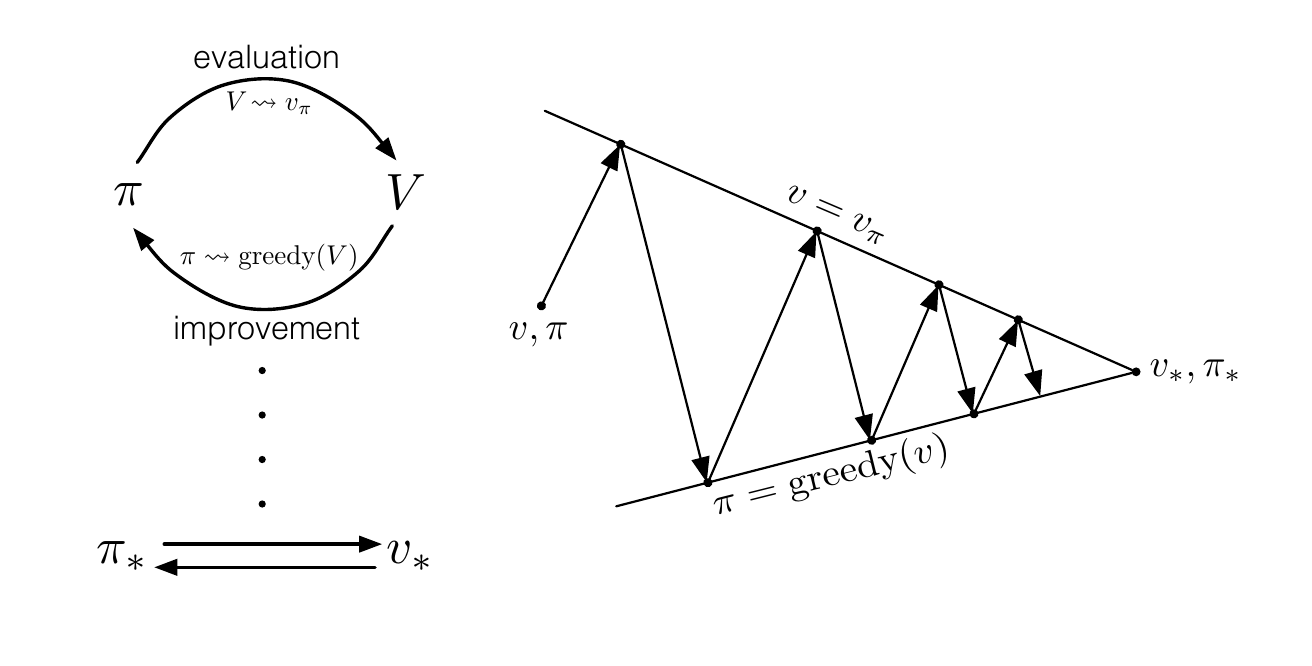
Our task really comes down to two tasks we can repeat over and over again to reach our optimal policy: we should be able to evaluate the current policy we are following and secondly, use this evaluation to improve our current policy. Formally, this is known as Generalized Policy Iteration (GPI).
Let’s Play!
Monte Carlo method
The term Monte Carlo is often used more broadly for any estimation method that relies on repeated random sampling. In RL Monte Carlo methods allow us to estimate values directly from experience, from sequences of states, actions and rewards. We use this as a way to evaluate the policy. Here we sample sequences of episodes: State, action, reward generated by following the policy till termination of the episode and the back propagate from the end to update the value of each state in the episode. The value of each state is the expected return from that state which can be calculated incrementally.
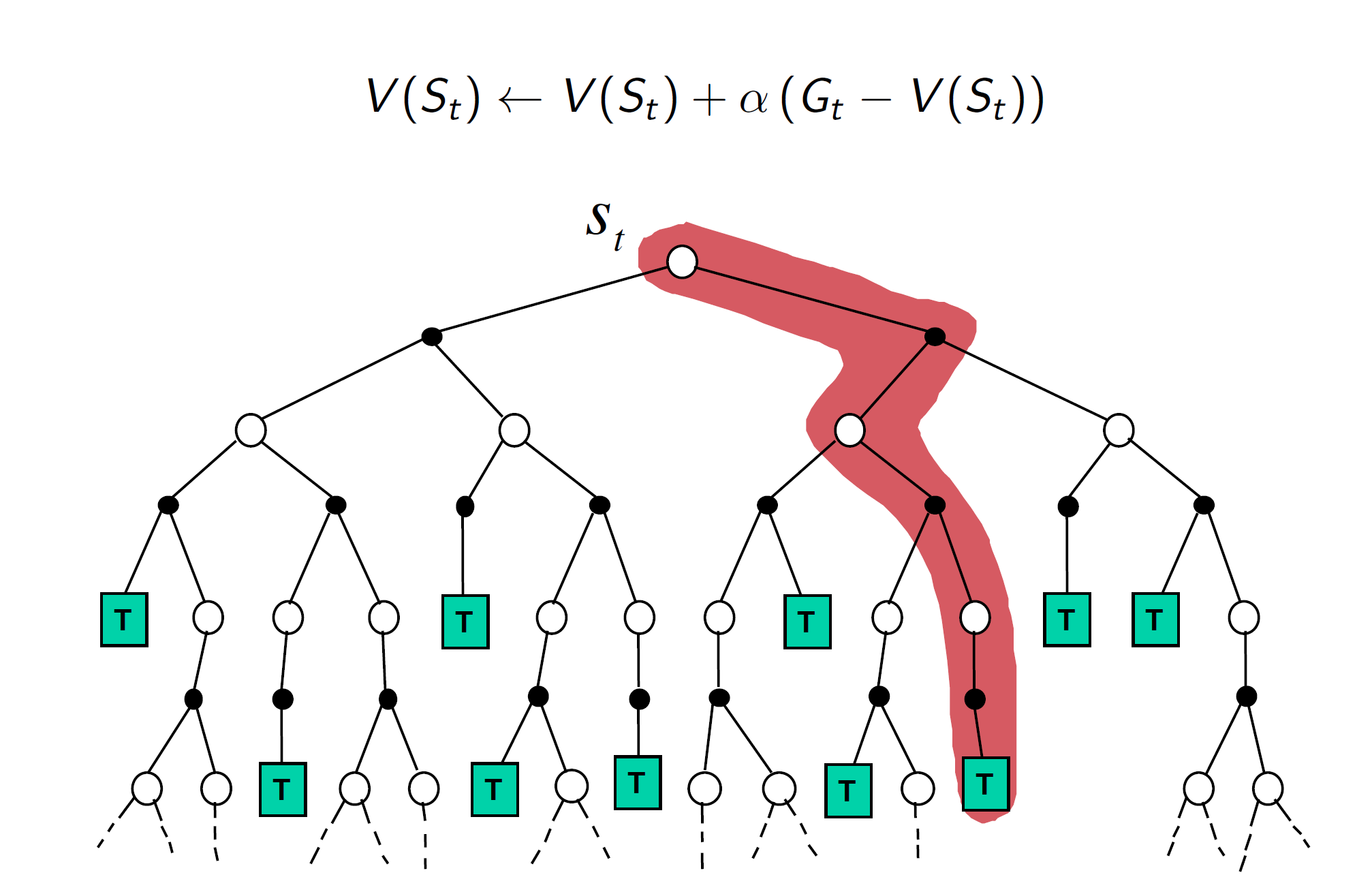
As an example, this is the evaluation of a policy that chooses to stick only on values of 20 or 21 (source: Sutton and Barto)
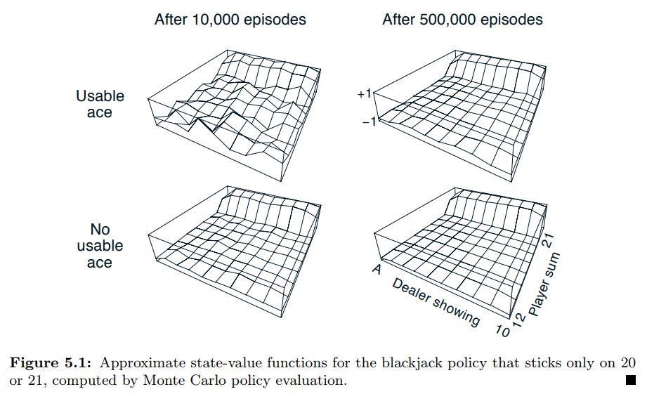
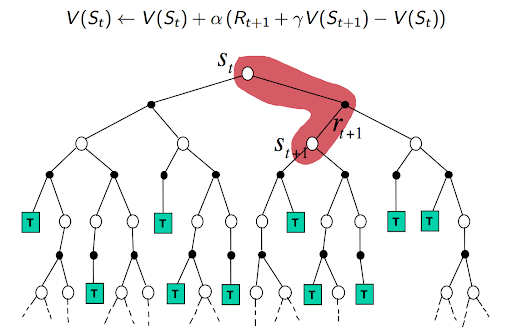
The game plan is to initialize our policy such that it’s stochastic which means that all actions have a possibility of being selected (here we just assign all probabilities to the same value or randomly initialize the policy). We evaluate the current policy using Monte Carlo evaluation and then we can easily improve this current policy but acting greedy with respect to it (we actually act ϵ greedily). Basically, look at the values corresponding to the current state in the Q-function and choose the action that maximizes the value. With this new policy, we re-compute the Q-table and the process goes on. Mathematically, going in reverse from the time step of termination of the episode, the return for each state-action pair is computed according to the following formula, with future rewards being discounted by a factor of γ raised to the power of how much later they are received. \(G_t=R_{t+1} + \gamma R_{t+2}+...+ \gamma ^{T-1}R_T\) Now the values are updated according to : \(Q(S,A)=Q(S,A)+ \alpha (G_t-Q(S,A))\) So the value is moved alpha (learning rate) times the error between what was previously computed to be the expected return and the return we actually received. To compute the returns, the value must be computed in reverse from the end of each episode. The backup diagram looks something like this:
The optimal policy learnt by this algorithm is as follows:
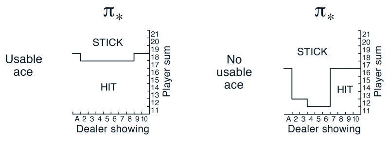 (source: Sutton and Barto)
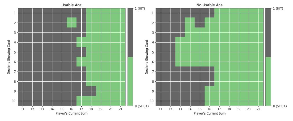
The agent we trained for 500,000 episodes with decaying epsilon value learnt the following policy:
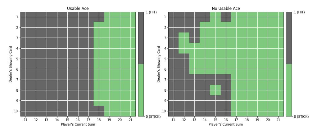
At a glance, it seems in the case of a usable ace, our agent learns a policy very similar to the HIT17 policy of our dealer. Since we can’t outright judge the quality of the policy, we observe the player playing 1000 rounds against the dealer and note the statistics.
wins = 434.0
draws = 89.0
losses = 477.0
However, we still can’t manage to beat the dealer but that isn’t too concerning here, since HIT17 is a pretty great policy to begin with and blackjack, like most casino games, is rigged to be in favor of the dealer. Regardless, if our agent learned a policy even slightly better than HIT17, it would have had more wins than losses.
DRAWBACKS OF MC
Monte Carlo methods inherently assume that the task you are using it on is episodic since it does wait till termination to update the Q-values. So, this algorithm can’t be applied to continuing tasks (for example, a personal assistant robot, its task doesn’t really have finite episodes and never ends). Additionally, say eventually on termination you got a big negative reward; this would affect the Q-values of all the states that came before in the episode, so the credit or blame isn’t assigned properly to certain states. While this may be fine for short episodic tasks like blackjack, for longer-horizon ones, it would be better to use temporal difference methods. Of these methods, here we will discuss Q-learning.
Before moving on, do note that blackjack is one of the cases where Monte Carlo works well given the nature of the environment. The game is episodic, each episode is short and the reward only appears at the end of the episode.
TEMPORAL DIFFERENCE METHODS
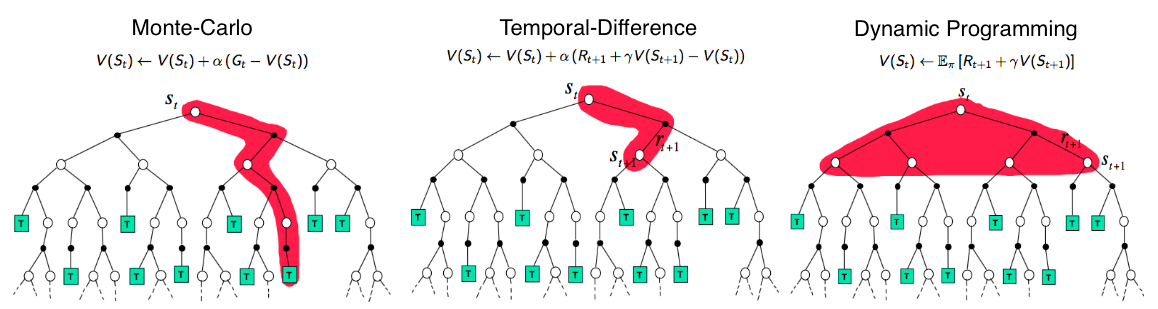
Temporal Difference (TD) methods bootstrap. What that fancy term means is that at each time step, it updates the values of each state by looking at the value of the next state (TD(0)) and working its way back. There are 3 methods under this: sarsa, Q-learning and expected-sarsa, of which we will assess Q-learning here. Here is a visual of what state or action values each method considers for backups
Q-learning
Here we use a similar initialization for Q-values for each state and action. We sample episodes and at each time step, the agent chooses an action ϵ-greedily, observes the reward from the next state and backs up the value for the current state-action pair. In Q-learning, in each step of each episode we sample, after choosing the action A and observing the reward R and next state S’, the action-value corresponding to S,A is updated according to the formula: \(Q(S,A)=Q(S,A)+ \alpha [R+ \gamma max(Q_a(S',a))-Q(S,A)]\) The difference between this and our previous monte carlo update is in the target for update. Previously it was the sampled return which was calculated in reverse from episode termination. Here the target is the reward received + the discount factor times the maximum value from the next state, out of all the possible actions from that state. This way, for each update, what is considered is the maximum over the action values of the next state. The backup diagram looks like this:
We once again train our agent on 500,000 episodes and it learns the following policy:
After 1000 games based on the above policy:
wins = 420.0
draws = 92.0
losses = 488.0
From these statistics, it does seem that our Q-learning policy didn’t perform as well as Monte Carlo; that could perhaps benefit from more rounds of training or tweaking the parameters. Regardless, temporal difference methods are usually more efficient and converge quicker since it updates the Q-values at every step and not just when an episode ends.
DRAWBACKS OF TD
Temporal difference learning is faster but less stable and may converge to the wrong solution. We estimate the Q-values only from the current reward, and use our own estimate of the values of the next state to predict the future reward. While this is faster, our targets are based on our estimation itself, making it unstable. Moreover, our estimate starts off arbitrarily wrong, so we might train toward wrong targets and might converge to a wrong solution.
What next?
There’s much more to learn of reinforcement learning and here we have seen a bit of the basics and watched the algorithms learn to play a relatively simple game. Achievements like AlphaGo were accomplished through even more complex methods and also using the brilliant idea of letting the agent play against itself to get better (self-play), which has played an important part in beating human level performance.
There are other similar applications where things get more complex, for instance, the number of states itself could be massive and computing values is infeasible. There are many methods to deal with this and various other situations. A lot of the work done in RL is relatively recent and much research is still on-going into the possibilities of its application.
There’s loads to explore (and exploit :p). Here are some resources to get you started: