The Math Behind Reinforcement Learning

Reinforcement learning is learning what to do, and how to map situations to actions, to maximize a numerical reward signal. The learner is not told which actions to take but instead must discover which actions yield the most reward by trying them. In the most interesting and challenging cases, actions may affect not only the immediate reward but also the next situation and, through that, all subsequent rewards. These two characteristics, trial-and-error search, and delayed reward are the two most important distinguishing features of reinforcement learning.

Markov Decision Process - The Environment

A Markov Decision Process is a set of rules that describe the environment for reinforcement learning to take place. Almost every task can be broken down into an MDP. In an MDP there are mainly three aspects:

• Agent: The learner and decision-maker
• Environment: The agent interacts with it; everything outside the agent; comprises states, which contain all the information for the agent to choose the best action in a given situation.
• Reward: Special numerical values given to the agent by the environment, the agent seeks to maximize this over time through its choice of actions. They can be positive or negative, describing desirable and undesirable actions respectively of an agent.

Every MDP must follow the Markov Property:

The state must include information about all aspects of the past agent–environment interaction that makes a difference in the future. i.e. the future is independent of the past given the present, and all information required to make decisions is given to the agent in the current state.

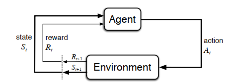
The agent and environment interact at each of a sequence of discrete-time steps, t = 0, 1, 2, 3, . . . . .

At each time step t, the agent receives some representation of the environment’s state, S_t ∈ S, and on that basis selects an action, A_t ∈ A(s). One time step later, in part as a consequence of its action, the agent receives a numerical reward, R_t ∈ R, and finds itself in a new state, S_t+1. The MDP and agent together thereby give rise to a sequence or trajectory that begins like this:

S₀, A₀, R₁, S₁, A₁, R₂, S₂, A₂, R₃, . . .

In a finite MDP, the sets of states, actions, and rewards (S, A, and R) all have a finite number of elements. In this case, the random variables R_t and S_t have well-defined discrete probability distributions dependent only on the preceding state and action. That is, for particular values of these random variables, s’ ∈ S and r ∈ R, there is a probability of those values occurring at time t, given particular values of the preceding state and action:

p(s’, r | s, a) = P {S_t = s’, R_t = r | S_t-1 = s, A_t-1 = a}

The above formula describes what is called the dynamics of an MDP, essentially it’s a conditional probability that tells us that upon taking an action in the state s what is the probability that we end up in the state s’ with a reward of r.

For every MDP the following should be true

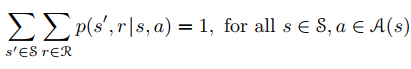
This tells us that for a state s and its set of actions a ∈ A(s), the probabilties set of exhausitve actions all add up.

Rewards and Discounting

The agent’s goal is to maximize the total amount of reward it receives. This means maximizing not immediate reward, but the cumulative reward in the long run.

Reward hypothesis:

That all of what we mean by goals and purposes can be well thought of as the maximization of the expected value of the cumulative sum of a received scalar signal (called reward).

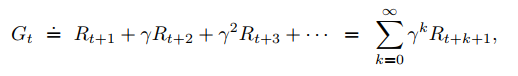
We seek to maximize the expected return, where the return, denoted G_t, is defined as some specific function of the reward sequence. In the simplest case the return is the sum of the rewards:

G_t =. R_t+1 + R_t+2 + R_t+3 + · · · + R_T

where T is a final time step.

However we quickly notice that just summing up all the rewards is cumbersome for the tasks which have long episode lengths, moreover, for continuous tasks, in which the task does not break down into natural sequences and goes on forever, the final time step R_T is not well defined to calculate return. Hence we use Discounting to overcome these challenges.

Using Discounting factor γ we can give the most immediate rewards more value than those that come later on. This makes sense intuitively as well, furthermore, it helps in breaking down tasks that don’t fall into discrete timesteps.

Policies

A policy is a mapping from states to probabilities of selecting each possible action. If the agent is following policy π at time t, then π(a|s) is the probability that A_t = a if S_t = s.(Note π is simply a probablitity function.)

Simply put a policy is the behavior of the agent, i.e. it tells us what actions the agent will take when presented a particular siutuation (state).

Value Functions

A value function tells us how good a particular state or state-action pair is for an agent. Value functions are always defined for a particular policy.

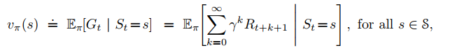
State Value function

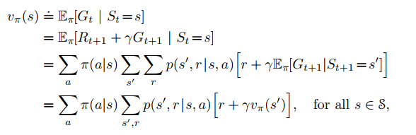
The value function of a state s under a policy π, denoted v_π(s), is the expected return when starting in s and following π thereafter.

Action Value function

value of taking action a in state s under a policy π, denoted v_π(s), is the expected return when starting in s and taking an action a, and following π thereafter.

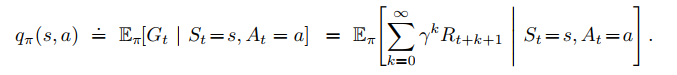here E denotes the expectation of a random variable

We can estimate the values of state function or action function using Monte Carlo methods, by averaging over many random samples of actual returns.

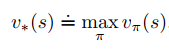
Optimal Policies and Optimal Value Functions

Solving a reinforcement learning task means, roughly, finding a policy that achieves a lot of rewards over the long run. For finite MDPs, we can precisely define an optimal policy in the following way. Value functions define a partial ordering over policies. A policy π is defined to be better than or equal to a policy π’ if its expected return is greater than or equal to that of π for all states. In other words, π ≥ π’ if and only if v_π(s) ≥ v_π’(s) for all s ∈ S. There is always at least one policy that is better than or equal to all other policies. This is an optimal policy. Although there may be more than one, we denote all the optimal policies by π^* . They share the same state-value function, called the optimal state-value function, denoted v^*

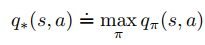
Optimal policies also share the same optimal action-value function.

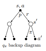
We can form backup diagrams to calculate both the state and action value functions.

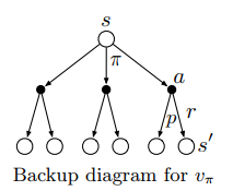
Bellman Equation

One fundamental property we exploit is that the value functions, can be represented as recursive calls, so they can be bootstrapped to the value of the previous state or state-action pair.

An intuitive example (Gridworld)

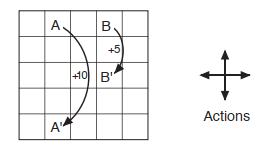
The below picture shows a rectangular gridworld representation of a simple finite MDP. The cells of the grid correspond to the states of the environment. At each cell, four actions are possible: north, south, east, and west, which deterministically cause the agent to move one cell in the respective direction on the grid. Actions that would take the agent off the grid leave its location unchanged, but also result in a reward of -1. Other actions result in a reward of 0, except those that move the agent out of the special states A and B. From state A, all four actions yield a reward of +10 and take the agent to A’. From state B, all actions yield a reward of +5 and take the agent to B’.

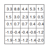
Suppose the agent selects all four actions with equal probability in all states.The below picture shows the value function, v_π(s), for this policy, for the discounted reward case with γ = 0.9. This value function was computed by solving the system of linear equations. Notice the negative values near the lower edge; these are the result of the high probability of hitting the edge of the grid there under the random policy. State A is the best state to be in under this policy, but its expected return is less than 10, its immediate reward because from A the agent is taken to A’, from which it is likely to run into the edge of the grid. State B, on the other hand, is valued more than 5, its immediate reward, because from B the agent is taken to B’, which has a positive value. From B’ the expected penalty (negative reward) for possibly running into an edge is more than compensated for by the expected gain for possibly stumbling onto A or B.

Using the Bellman equation for the same Grid World for v ^* and solving the set of linear equations that are obtained thereafter we get the optimal policy π^*. The picture below shows the optimal value function and the corresponding optimal policies. Where there are multiple arrows in a cell, all of the corresponding actions are optimal.

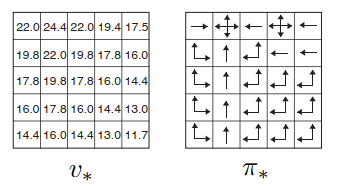
You may notice that there is more than one optimal action the agent can take in a particular given state, this leads to more than one optimal policy. However, the optimal value function is unique for a given task/environment.

You may notice that there is more than one optimal action the agent can take in a particular given state, this leads to more than one optimal policy. However, the optimal value function is unique for a given task/environment.

There are multiple methods to obtain the optimal value functions, and based on these multiple reinforcement learning algorithms have been proposed. For example, in Monte-Carlo methods, the value function is determined by taking repeated samples via experience and then averaging them. These kinds of algorithms perform well when the dynamics of the environment is not given to us. Other methods use two policies, one for exploring the environment and another for updating the value functions, these methods are called off-policy methods as they learn the optimal policy regardless of the agent’s motivation. Similarly, we can find different algorithms that perform well in different situations, I suggest that you explore these for yourself.

This is the fundamental math behind Reinforcement Learning. Based on the situation we exploit different fundamental math properties and use the formulas to our advantage.

If you think about it reinforcement learning is rote learning for computers.

References

1. Reinforcement learning - Wikipedia
2. Richard S. Sutton and Andrew G. Barto. Reinforcement Learning: An Introduction, Second edition. The MIT Press, Cambridge Massachusetts, 2018.