LSTM Models

What’s the first thing that comes to your mind when you think of speech recognition? Alexa, Google assistant, Cortana, right? It’s quite reasonable; we are fascinated by machines that can understand us. But have you ever wondered how these things even work? As you read this article, you’ll get the basic idea along with the maths used behind this.

When analyzing human voice, a very important aspect are filters, which constitute a selective frequency transmission system that allows energy through some frequencies and not others. Currently, the standard way of preprocessing audio is to compute the short-time Fourier transform (STFT) with a given hop size from the raw waveform. This gives us a tridimensional arrangement called a spectrogram that shows the frequency distribution and intensity of the audio as a function of time.

Once we have the spectrogram, it is possible to propose a neural network that is able to handle command recognition while still keeping a small footprint in terms of number of trainable parameters. This leads to our main topic of the article, LSTM models. But before going to that, let’s just look at its predecessor model, Recurrent Neural Network (RNN).

Recurrent Neural Networks

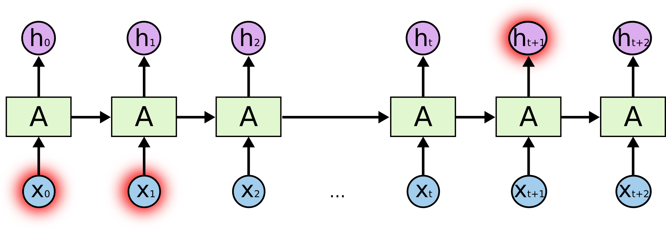
Humans don’t start their thinking from scratch every second. As you are reading this essay, you understand each word based on your understanding of previous words. You don’t throw everything away and start thinking from scratch again. Your thoughts have persistence. Traditional neural networks can’t do this, and it seems like a major shortcoming. Recurrent neural networks address this issue. They are networks with loops in them, allowing information to persist.

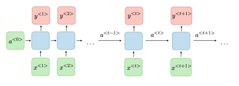
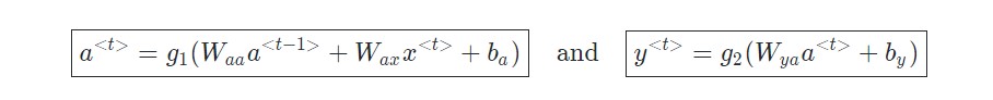
Recurrent neural networks (RNNs), are a class of neural networks that allow previous outputs to be used as inputs while having hidden states. It can be thought of as multiple copies of the same network, each passing a message to a successor. For each timestamp t, the activation a and the output y are expressed as follows:

where Wax , Waa , Wya , ba , by are the coefficients that are shared temporally and g1 , g2 activation functions.

The Problem of Long-Term Dependencies

RNNs were designed to connect the previous information to the present task, but unfortunately, as the gap grows, RNNs become unable to connect the information.

The reason behind this behavior is vanishing and exploding gradients. Due to this, it is difficult to capture long-term dependencies because of multiplicative gradients that can be exponentially decreasing/increasing with respect to the number of layers.

Thankfully, LSTMs don’t have this problem!

LSTM Networks

Long Short Term Memory (LSTMs) are explicitly designed to avoid the vanishing and exploding gradient phenomenon. They have internal mechanisms called gates that can regulate the flow of information. Like RNNs, LSTMs also have a chain-like structure, but the repeating module has a different structure. Instead of having a single neural network layer, there are four layers that interact in a very special way.

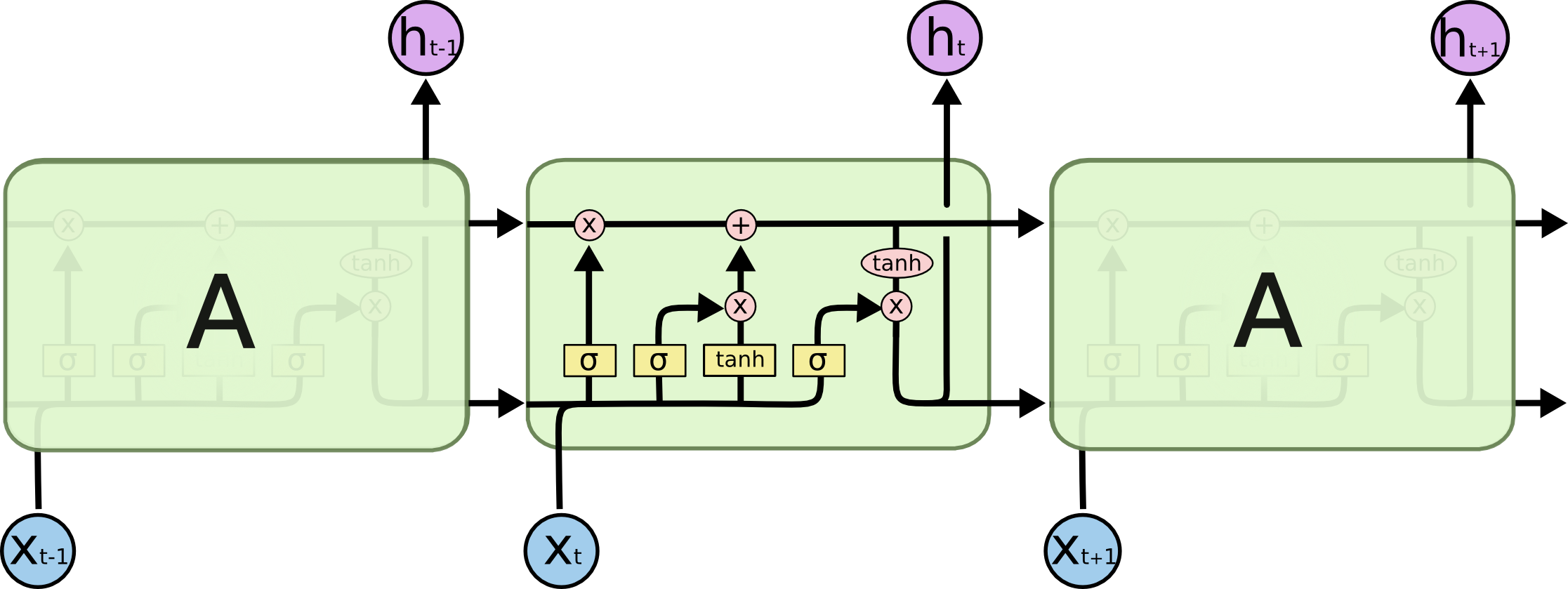
First of all, let’s just try to get comfortable with the notation we’ll be using.

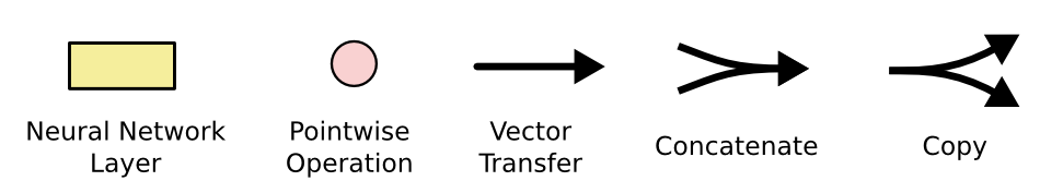
In the above diagram, the pale yellow boxes represent a neural network layer. The pink circles represent pointwise operations, like vector addition/subtraction. Lines merging denote concatenation, while a line forking denotes its content being copied and the copies are passed to different locations.

The Core Idea Behind LSTMs

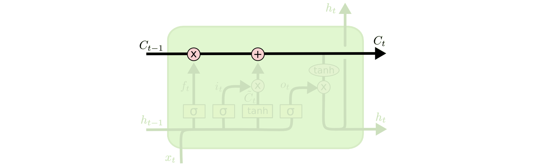
The core concept of LSTMs are the cell states and its various gates. One can treat cells like a conveyor belt. It runs straight down the entire chain, with only some minor linear interactions which helps to retain info even in a very long chain. It’s very easy for information to just flow along it unchanged.

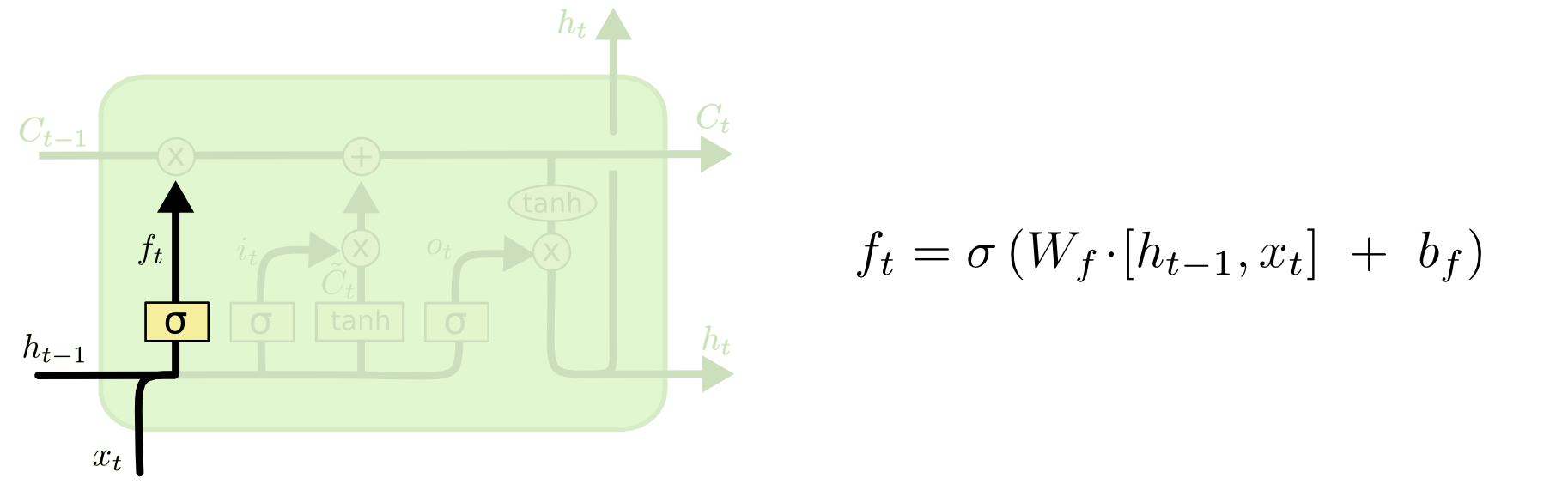
Gates provides a way to optionally let information through. They’re composed of a sigmoid neural network layer and a pointwise multiplication operation. First, we’ve the “forget gate”. This gate decides what information should be kept or thrown away. Data from the current input is passed through the sigmoid function. Values come out to be 0 and 1. The values that are closer to 0 means to forget and closer to 1 means to keep.

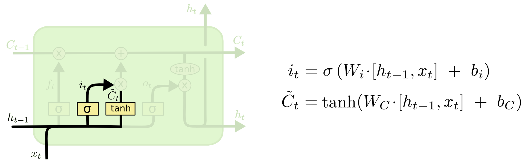
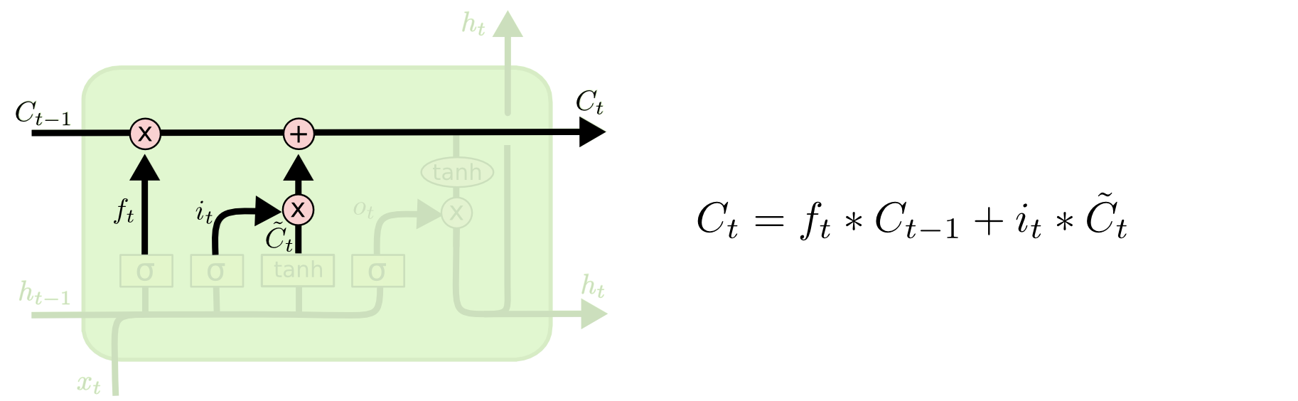
Next, we’d like to make a decision on what new information we’re going to store within the cell state. This has two parts. First, a sigmoid layer also called the “input gate layer” decides which values we’ll update. Next, a tanh layer creates a vector of the latest candidate values, C~t, that would be added to the state. In the next step, we’ll combine these two to make an update to the state.

It’s now time to update the old cell state, Ct−1, into the new cell state Ct. This is the new candidate value, scaled by how much we decided to update each state value.

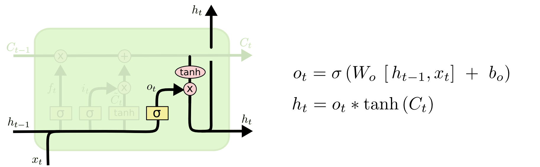
Finally, we have the output gate which will output a filtered version of the cell state. First, we have a sigmoid layer which decides the parts of the cell state we’re going to output. Then, we put the cell state through tanh which ensures to keep the values between 1 and -1, and then, multiply it by the output of the sigmoid gate, so that we can get desirable output.

Applications of LSTMs

Language Modelling and predictions

In this method, the likelihood of a word in a sentence is considered. The probability of the output of a particular time-step is used to sample the words in the next iteration(memory). In Language Modelling, input is usually a sequence of words from the data and output will be a sequence of predicted word by the model. While training we set xt+1 = ot, the output of the previous time step will be the input of the present time step.

Speech Recognition

A set of inputs containing phoneme(acoustic signals) from an audio is used as an input. This network will compute the phonemes and produce a phonetic segments with the likelihood of output.

Machine Translation

In Machine Translation, the input is will be the source language(lets say Hindi) and the output will be in the target language(lets say English). The main difference between Machine Translation and Language modelling is that the output starts only after the complete input has been fed into the network.

Conclusion

We have learned the basic idea behind RNN and LSTM, how LSTM manages the shortcomings of RNN and their use in speech recognition. LSTMs are a very promising solution to sequence and time series related problems. Within a few dozen minutes of training can generate nice looking descriptions of images, Image Captioning. LSTM’s and GRU’s are also used in state-of-the-art deep learning applications like speech synthesis, natural language understanding, etc.

If you’re interested in going deeper, here are links to some fantastic resources that can give you a different perspective in understanding LSTM’s and GRU’s. This post was heavily inspired by them.