I’d like to talk about an algorithm that I believe should be in any Software Engineer’s toolkit. That is, the KMP algorithm named after its three inventors: Knuth-Morris-Pratt. The algorithm was designed to solve efficiently a very common problem. That is the problem of finding whether or not one string is a substring of a different string.
Brute Force
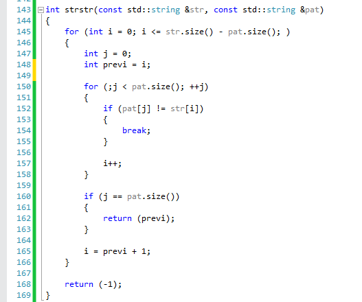
Let’s start first with the original problem. We would like to implement the function: int strstr(const string &Str, const string& Pattern); The brute force solution of this function entails two loops, one over Str and one over pattern. Let’s see it:
What is the runtime complexity of this algorithm?
Since we are running in two loops and for each i we are trying all j’s, we have a worst-case complexity of O(NM) where N is the size of Str and M is the size of Pat. Can you spot where the inefficiency comes from? The problem is that if we can’t find a match we have to go back (with i) and start over from where we left off when we started the match. Why are we doing this? let’s look at two examples:
-
str = “abcbcefg” and pat = “bce”. In this case we start the match at i = 1 and j = 0, we continue to i = 2 and j = 1, but then at i = 3 and j = 2 we have a mismatch. Our algorithm will detect this mismatch and will set “i” to be 2. But what’s the point? for i = 2 we already know that there will be no match. In fact, based on strwe should not be setting “i” to a previous index, but we could just as well continue advancing i.
-
str = “abababc” pat = “ababc”. In this case, we will start matching at i = 0 and will reach i = 4 when we detect a mismatch. We will then return to i = 1 and start again. When we reach i = 2 we will detect that the strings match. The observation is, that we should not have even bothered returning to i = 1 we could have set “i”to 2. But, if we look even closer we may notice that after we matched str = “abab” and pat = “abab” we already have one pair of “ab” in pat which we know that can be used for future matches.
Let’s try and make our code efficient!
The two examples are a great way to explain how KMP works and why it is so efficient. KMP starts off by building a prefix table for pat. This prefix table will be used to indicate for each index “i” how much we have matched thus far and use this information to jump back only by the amount needed.
Lets see how the prefix table will look like for different patterns:
- pat = “ababc” will result in the table: {0,0,1,2,0}
- pat = “ississi” will result in the table: {0,0,0,1,2,3,4}
- pat = “abcd” will result in the table: {0,0,0,0}
Notice what is happening here. When we detect a prefix that we have seen (such as the second “ab” in “ababc”) the numbers in the table indicate the size of that prefix. So if we start matching “abababc” with “ababc” for i = 4 and j = 4 we see that ‘a’ is different from ‘c’, and hence we have a mismatch. Using the table above we see that the table at index j - 1 = 3 has the value 2. We can have “j” jump back two indexes from 4 to 2, and continue our match from there. We don’t have to touch “i” anymore, we just modify “j” based on the maximal size of the prefix that we have seen thus far.
Let us see the code to generate the Prefix table:
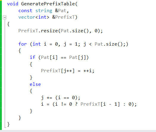
We allocate the prefix table to be the size of “Pat”. We use two indexes to fill the table. The first is “i”, it will indicate the end of the current prefix. The second is “j” which will be used to find the next occurance of the prefix. Notice that “j” starts from index 1. As we are traversing we check to see whether Pat[i] == Pat[j]. If they are, then we know that there is a prefix of size i + 1 that we have encountered at index “j”. We update the table at index “j” to indicate this prefix, and update “i” as well. If they are not the same, then we have two cases: First, if i == 0, it means that we have not found any prefix thus far and we just increment “j”. However, if i > 0, we keep “j” where it is and make “i” go back to the index where the prefix has started and compare it again with “j” .
Complete code
We are now ready to see the full algorithm and how it uses the prefix table:
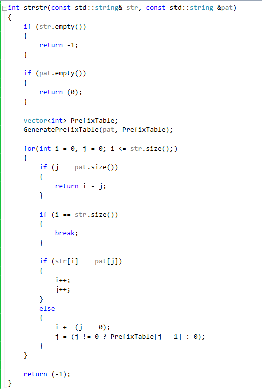
The runtime complexity of this new version in the worst case will be O(N).