![]()
An Introduction to PyTorch
PyTorch was released in early 2017 by Adam Paszke, Sam Gross, Soumith Chintala, Gregory Chanan and has been making a pretty big impact in the deep learning community. It's is a Python-based scientific computing package targeted to be a: (1) A replacement for NumPy to use the power of GPUs and (2) A deep learning research platform that provides maximum flexibility and speed. It's developed as an open source project by the Facebook AI Research team, and is being adopted by teams everywhere in industry and academia and is very comfortable to learn and use. It is based on the Torch library and has both a Python and C++ frontend(though the Python frontend is more 'polished'). PyTorch is also very pythonic, meaning, it feels more natural to use it if you already are a Python developer.
What we'll see
In this post, we will first look at the basics of Tensors(which are the building blocks of anything you do using PyTorch), and operations on them. We will then have a look at gradients and how they are computed in PyTorch. Finally we shall build a simple Neural Network for the IRIS dataset using PyTorch
Prerequisites
Knowledge of Python(3.x) is required. Knowledge of NumPy will be useful but is not necessary. For the last part (of building a Neural Network), a basic understanding of a simple neural network is assumed
Installation
Details of installation may be found here. However, to start off with, I would recommend using Google Colab or Microsoft Azure
We'll first have a look at the building blocks of PyTorch (most other deep learning libraries also) which are Tensors.
Tensors
All computations in PyTorch generally consist of operations on Tensors. Tensors can be thought of as a generalisation of vectors or matrices in 1 or more dimensions, or more simply, are like arrays in a programming language like C. In some cases tensors are used as a replacement for NumPy to use the power of GPUs A 1D Tensor is like a 1D array, 2D Tensor like a 2D array and so on. Let’s see how we can use them.
Importing torch
import torch
torch.__version__
'1.1.0'
Tensors are available in the torch library as torch.Tensor. It is like a multidimensional array which can have elements of a single datatype. Computations between tensors are allowed only if the tensors share the same data type(dtype).
First lets create a tensor from a python list:
myTensor = torch.tensor([1, 2, 3])
myTensor
tensor([1, 2, 3])
myTensor1 = torch.tensor([[1, 2, 3.0], [4, 5, 6]])
myTensor1
tensor([[1., 2., 3.],
        [4., 5., 6.]])
Above, we see that the function determines the data type based on the inputs. We may use different constructors to specify the data type we need as:
fltTensor = torch.FloatTensor([1, 2, 3])
fltTensor
tensor([1., 2., 3.]) <br>
intTensor = torch.IntTensor([1.0, 2.0, 3])
intTensor
tensor([1, 2, 3], dtype=torch.int32) <br>
longTensor = torch.LongTensor([1.0, 2, 3])
longTensor
tensor([1, 2, 3])
We may also achieve the above using the dtype attribute in torch.tensor:
intTensor1 = torch.tensor([1.0, 2.0, 3], dtype = torch.int)
intTensor1
tensor([1, 2, 3], dtype=torch.int32)
Note: There is a subtle difference between the functions torch.tensor and torch.Tensor. torch.Tensor is an alias to torch.FloatTensor whereas torch.tensor determines the data type based on the input.
For more information on datatypes, check here.
To and From a NumPy array
Converting a torch tensor to a numpy array and vice versa is very easy and hence makes it easy to access other libraries like Scikit-Learn and Matplotlib
import numpy as np
arr = np.array([1,2,3,4,5])
print(arr)
print(arr.dtype)
print(type(arr))
[1 2 3 4 5]
int32
<class 'numpy.ndarray'>
We can use torch.from_numpy or torch.as_tensor:
x = torch.from_numpy(arr)
x
tensor([1, 2, 3, 4, 5], dtype=torch.int32)
print(type(x))
print(x.type())
<class 'torch.Tensor'>
torch.IntTensor
Note that we can also use torch.tensor for this:
x1 = torch.tensor(arr)
x1
tensor([1, 2, 3, 4, 5], dtype=torch.int32)
The difference between torch.tensor and torch.from_numpy(or torch.as_tensor) is that when we use the former, a copy of the original tensor is made and stored in x1(above). Any changes made to x1 will not affect arr(the numpy array) and vice versa. However, when we use the latter function, the tensor created (x in the example above) points to the same location in memory as does arr. Hence any changes done to x will also affect arr(the numpy array) and vice versa.
# Using torch.from_numpy()
arr = np.arange(0,5)
t = torch.from_numpy(arr)
arr[2]=100
print(t)
tensor([ 0, 1, 100, 3, 4], dtype=torch.int32)
# Using torch.tensor()
arr = np.arange(0,5)
t = torch.tensor(arr)
arr[2]=100
print(t)
tensor([0, 1, 2, 3, 4], dtype=torch.int32)
Creating special types of tensors
Uninitialized tensors using torch.empty()
x = torch.empty(5, 4)
print(x)
tensor([[0., 0., 0., 0.],
        [0., 0., 0., 0.],
        [0., 0., 0., 0.],
        [0., 0., 0., 0.],
        [0., 0., 0., 0.]])
Initialised with zeroes or ones using torch.zeros() and torch.ones()
# Passing datatype is recommended but not compulsory
x = torch.zeros(4, 3, dtype=torch.int64)
print(x)
tensor([[0, 0, 0],
        [0, 0, 0],
        [0, 0, 0],
        [0, 0, 0]])
Tensors in a range using torch.arange(start,end,step) and torch.linspace(start,end,number_of_elements)
x = torch.arange(0,50,5).reshape(5,2) # 0 included, 50 excluded
print(x)
tensor([[ 0,  5],
        [10, 15],
        [20, 25],
        [30, 35],
        [40, 45]])
Tensor to create 12 linearly spaced elements between 0 and 50 both included
x = torch.linspace(0,50,12).reshape(3,4)
print(x)
tensor([[ 0.0000,  4.5455,  9.0909, 13.6364],
        [18.1818, 22.7273, 27.2727, 31.8182],
        [36.3636, 40.9091, 45.4545, 50.0000]])
A seed for random numbers can be set using torch.manual_seed().
torch.manual_seed(10)
<torch._C.Generator at 0x1bb6e171030>
Generating random tensors:
A tensor of shape (3, 4) with random numbers from a uniform distribution over [0, 1)
x = torch.rand(3, 4)
x
tensor([[0.9712, 0.0742, 0.5130, 0.7472],
        [0.4507, 0.9223, 0.9148, 0.1624],
        [0.7780, 0.1663, 0.6665, 0.4992]])
A tensor with shape (3, 4) with numbers from the normal distribution with mean 0 and standard deviation 1.
x = torch.randn(3, 4)
x
tensor([[ 0.5252,  2.0810,  1.5700, -0.1474],
        [-0.2024,  0.4377,  1.1986,  0.7179],
        [-0.4969,  0.8618, -0.2603, -1.1157]])
A tensor of shape (3, 4) with random integers between 0 and 10
x = torch.randint(0, 10, (3, 4))
x
tensor([[7, 7, 1, 4],
        [7, 4, 9, 5],
        [1, 2, 5, 6]])
Instead of specifying the sizes of the tensors, we can use three other functions which serve the same purpose as above nute take in other tensors as inputs and return tensors of their shapes. Just suffix _like to the above functions as below:
x = torch.rand(3, 4)
y = torch.rand_like(x)
y
tensor([[0.3099, 0.0135, 0.2955, 0.8752],
        [0.7608, 0.7589, 0.2097, 0.4063],
        [0.6469, 0.3655, 0.3926, 0.6284]])
Similarly torch.randn_like(x), torch.randint_like(0,10,x), torch.zeros_like(x) and torch.ones_like(x) may also be used.
Operations on Tensors
Now we will look at a few basic operations on Tensors. Indexing and slicing tensors are very similar to those of python lists. We shall look at a few examples
x = torch.arange(6).reshape(3,2)
print(x)
tensor([[0, 1],
        [2, 3],
        [4, 5]])
To get the left column:
x[:,0]
tensor([0, 2, 4])
To get the left column as a (3,1) slice:
x[:,:1]
tensor([[0],
        [2],
        [4]])
Reshaping a Tensor
Two functions are generally used for reshaping tensor which are .view() and .reshape(). Both functions return a reshaped tensor without affecting the original tensor.
x = torch.arange(10)
x
tensor([0, 1, 2, 3, 4, 5, 6, 7, 8, 9]) <br>
x.view(5, 2)
tensor([[0, 1],
        [2, 3],
        [4, 5],
        [6, 7],
        [8, 9]])
However, we see that x is unchanged
x
tensor([0, 1, 2, 3, 4, 5, 6, 7, 8, 9])
x.reshape(5, 2)
tensor([[0, 1],
        [2, 3],
        [4, 5],
        [6, 7],
        [8, 9]]) <br>
x # Unchanged
tensor([0, 1, 2, 3, 4, 5, 6, 7, 8, 9])
To change the original tensor use x = x.reshape(2, 5)
While .view() returns a tensor which shares storage with the original tensor, .reshape() may return a copy or a view of the original tensor. It (.reshape()) may or may not share the storage with the original tensor. Also .reshape() may act on contiguous or non contiguous tensors, while .view can act only on contiguous tensors.
We can also infer the correct value for shape from the tensor by passing -1.
x = x.view(2, -1)
x
tensor([[0, 1, 2, 3, 4],
        [5, 6, 7, 8, 9]])
Also as seen before, we can suffix the function with ‘_as’ to pass in a tensor whose shape, we want to reshape the original tensor to.
y = torch.arange(0, 20, 2)
y
tensor([ 0, 2, 4, 6, 8, 10, 12, 14, 16, 18])
y = y.view_as(x)
y
tensor([[ 0,  2,  4,  6,  8],
        [10, 12, 14, 16, 18]])
Other Basic Operations
I will demonstrate the use of basic operations using the torch.add() function. This may be extended to other functions also.
a = torch.tensor([1,2], dtype=torch.float)
b = torch.tensor([3,4], dtype=torch.float)
print(a + b)
tensor([4., 6.])
torch.add(a, b)
tensor([4., 6.])
c = torch.empty(2)
torch.add(a, b, out = c) #Equivalent to c = torch.add(a, b)
tensor([4., 6.])
a.add_(b) #Equivalent tp a = torch.add(a,b)
a
tensor([4., 6.])
The above can be extended to all basic arithmetic operations. Now we will look at a few more operations
# Multiplication (element-wise)
a = torch.tensor([1,2], dtype=torch.float)
b = torch.tensor([3,4], dtype=torch.float)
torch.mul(a, b)
tensor([3., 8.])
# Dot Product
torch.dot(a, b)
tensor(11.)
Now let us see matrix multiplication. Normal matrix multiplication (that we know of) can be done using torch.mm()
a = torch.tensor([[0,2,4],[1,3,5]], dtype=torch.float)
b = torch.tensor([[6,7],[8,9],[10,11]], dtype=torch.float)

print('a: ',a.size())
print('b: ',b.size())
print('a x b: ',torch.mm(a,b).size())
a:  torch.Size([2, 3])
b:  torch.Size([3, 2])
a x b:  torch.Size([2, 2])
torch.mm(a,b)
tensor([[56., 62.],
        [80., 89.]])
a @ b
tensor([[56., 62.],
        [80., 89.]])
Matrix multiplication can also be done with boradcasting using the torch.matmul() or @ operator. Click here for more details on broadcasting.
a = torch.randn(2, 3, 4)
b = torch.randn(4, 5)

print(torch.matmul(a, b).size())
print((a @ b).size())
torch.Size([2, 3, 5])
torch.Size([2, 3, 5])
But we see that there matrices are invalid for normal matrix multiplication
print(torch.mm(a,b))
---------------------------------------------------------------------------

RuntimeError                              Traceback (most recent call last)

<ipython-input-93-244d2942b50e> in <module>
----> 1 print(torch.mm(a,b))


RuntimeError: matrices expected, got 3D, 2D tensors at ..\aten\src\TH/generic/THTensorMath.cpp:956
Note that if the tensors satisfy the mathematical conditions of matric multiplication, then all the three above functions will be identical. It is however easier to detect errors using torch.mm() than the other two when the tensors are mathematically non-compatible and hence is recommended over the other two.
Norm Function
x = torch.tensor([2.,5.,8.,14.])
x.norm()
tensor(17.)
Gradients in PyTorch
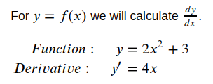
PyTorch provides a module called ‘autograd’ to calculate the gradients of tensors automatically. It basically keeps track of all operations done on the tensor and backtracks along these operations to calculate gradients(or derivatives) along the way. To ensure that the operations are kept track of, we need to set the requires_grad attribute to True which can be done in two ways: (1) while creation, set the attribute to True as x = torch.arange(10, requires_grad = True) or (2) after creation, use x.requires_grad_(True). The gradients are computed with respect to some variable y as y.backward(). This goes though all operations which were used to create y and calculates the gradients. For example:
x = torch.tensor(3.0, requires_grad = True)
y = 2 * x ** 2 + 3
print(y) # Substitutes the value of x = 3 in the equation
tensor(21., grad_fn=<AddBackward0>)
#Perform backpropagation on y to calculate gradients
y.backward()
#Display the gradient wrt x
x.grad
tensor(12.)
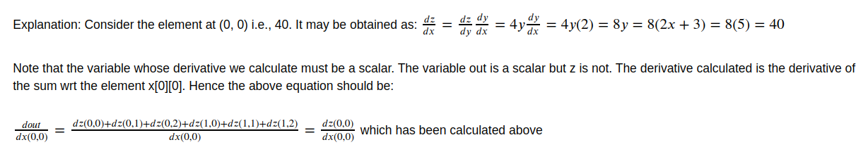
Calculating multi-level gradients
x = torch.tensor([[1.,2,3],[3,2,1]], requires_grad=True)
print(x)
tensor([[1., 2., 3.],
        [3., 2., 1.]], requires_grad=True)
y = 2*x + 3
print(y)
tensor([[5., 7., 9.],
        [9., 7., 5.]], grad_fn=<AddBackward0>)
z = 2*y**2
print(z)
tensor([[ 50.,  98., 162.],
        [162.,  98.,  50.]], grad_fn=<MulBackward0>)
out = z.sum()
print(out)
tensor(620., grad_fn=<SumBackward0>)
out.backward()
print(x.grad)
tensor([[40., 56., 72.],
        [72., 56., 40.]])
Turning off tracking
There may be times when we don’t want or need to track the computational history.
You can reset a tensor’s requires_grad attribute in-place using .requires_grad_(True) (or False) as needed.
When performing evaluations, it’s often helpful to wrap a set of operations in with torch.no_grad():
A less-used method is to run .detach() on a tensor to prevent future computations from being tracked. This can be handy when cloning a tensor.
Building a Simple Neural Network
Note that the rest of the article will need some knowledge of Machine Learning or Neural Networks.
We will discover other features like Dataloaders, Criterions and Optimizers using an example on the IRIS Dataset
import pandas as pd
import numpy as np
import torch

df = pd.read_csv('iris.csv')
df.head()
| sepal length (cm) | sepal width (cm) | petal length (cm) | petal width (cm) | target | |
|---|---|---|---|---|---|
| 0 | 5.1 | 3.5 | 1.4 | 0.2 | 0.0 |
| 1 | 4.9 | 3.0 | 1.4 | 0.2 | 0.0 |
| 2 | 4.7 | 3.2 | 1.3 | 0.2 | 0.0 |
| 3 | 4.6 | 3.1 | 1.5 | 0.2 | 0.0 |
| 4 | 5.0 | 3.6 | 1.4 | 0.2 | 0.0 |
PyTorch has 2 really useful libraries for Neral Networks:
- torch.nn generally imported as nn
- torch.nn.functional generally imported as F
import torch.nn as nn
import torch.nn.functional as F
from torch.utils.data import Dataset, DataLoader, TensorDataset
from sklearn.model_selection import train_test_split
X = df.drop('target',axis=1).values
y = df['target'].values

X_train, X_test, y_train, y_test = train_test_split(X,y,test_size=0.2,random_state=100)

X_train = torch.FloatTensor(X_train)
X_test = torch.FloatTensor(X_test)

# One Hot Encoding
y_train = torch.LongTensor(y_train)
y_test = torch.LongTensor(y_test)
To convert the training tensors into a dataset and to make things like batch gradient descent easier, we may use the TensorDataset and DataLoader classes.
trainset = TensorDataset(X_train, y_train)
We will create batches of size 30. We will shuffle the training data so that the batches are not biased. However this is not necessary for the test data.
trainloader = DataLoader(trainset, batch_size=30, shuffle=True)
testloader = DataLoader(X_test, batch_size=30, shuffle=False)
To access the batches:
# 4 batches. Each batch is two-dimensional, one for the features(X) and other for the classes(y).
for batch in trainloader:
    print(len(batch))
2
2
2
2
# To access the index, X data and Y data
for i, (x,y) in enumerate(trainloader):
    print(i, x, y)
    print()
0 tensor([[5.7000, 2.9000, 4.2000, 1.3000],
        [7.4000, 2.8000, 6.1000, 1.9000],
        [6.9000, 3.1000, 5.1000, 2.3000],
        [5.3000, 3.7000, 1.5000, 0.2000],
        [5.4000, 3.0000, 4.5000, 1.5000],
        [5.5000, 4.2000, 1.4000, 0.2000],
        [6.1000, 2.6000, 5.6000, 1.4000],
        [5.5000, 2.6000, 4.4000, 1.2000],
        [6.0000, 3.4000, 4.5000, 1.6000],
        [5.7000, 2.5000, 5.0000, 2.0000],
        [4.4000, 3.2000, 1.3000, 0.2000],
        [5.0000, 3.6000, 1.4000, 0.2000],
        [4.9000, 3.1000, 1.5000, 0.1000],
        [7.0000, 3.2000, 4.7000, 1.4000],
        [6.3000, 2.5000, 4.9000, 1.5000],
        [6.1000, 2.8000, 4.0000, 1.3000],
        [6.5000, 3.0000, 5.8000, 2.2000],
        [5.1000, 3.8000, 1.5000, 0.3000],
        [5.0000, 3.0000, 1.6000, 0.2000],
        [4.6000, 3.6000, 1.0000, 0.2000],
        [5.7000, 2.8000, 4.5000, 1.3000],
        [4.9000, 3.1000, 1.5000, 0.1000],
        [5.8000, 2.7000, 4.1000, 1.0000],
        [5.1000, 3.3000, 1.7000, 0.5000],
        [4.4000, 2.9000, 1.4000, 0.2000],
        [6.2000, 2.2000, 4.5000, 1.5000],
        [7.9000, 3.8000, 6.4000, 2.0000],
        [7.7000, 3.8000, 6.7000, 2.2000],
        [6.3000, 2.9000, 5.6000, 1.8000],
        [5.5000, 2.5000, 4.0000, 1.3000]]) tensor([1, 2, 2, 0, 1, 0, 2, 1, 1, 2, 0, 0, 0, 1, 1, 1, 2, 0, 0, 0, 1, 0, 1, 0,
        0, 1, 2, 2, 2, 1])

1 tensor([[5.0000, 3.2000, 1.2000, 0.2000],
        [4.9000, 3.1000, 1.5000, 0.1000],
        [6.7000, 3.3000, 5.7000, 2.1000],
        [5.5000, 3.5000, 1.3000, 0.2000],
        [5.4000, 3.9000, 1.7000, 0.4000],
        [6.0000, 3.0000, 4.8000, 1.8000],
        [5.1000, 2.5000, 3.0000, 1.1000],
        [5.9000, 3.0000, 4.2000, 1.5000],
        [7.6000, 3.0000, 6.6000, 2.1000],
        [6.4000, 2.7000, 5.3000, 1.9000],
        [5.1000, 3.8000, 1.6000, 0.2000],
        [6.9000, 3.1000, 5.4000, 2.1000],
        [7.2000, 3.6000, 6.1000, 2.5000],
        [5.1000, 3.5000, 1.4000, 0.2000],
        [6.5000, 3.2000, 5.1000, 2.0000],
        [5.5000, 2.4000, 3.7000, 1.0000],
        [5.6000, 2.8000, 4.9000, 2.0000],
        [6.3000, 3.4000, 5.6000, 2.4000],
        [7.3000, 2.9000, 6.3000, 1.8000],
        [5.9000, 3.2000, 4.8000, 1.8000],
        [6.8000, 2.8000, 4.8000, 1.4000],
        [4.9000, 2.5000, 4.5000, 1.7000],
        [5.1000, 3.5000, 1.4000, 0.3000],
        [6.2000, 3.4000, 5.4000, 2.3000],
        [5.7000, 2.8000, 4.1000, 1.3000],
        [6.1000, 3.0000, 4.9000, 1.8000],
        [5.5000, 2.4000, 3.8000, 1.1000],
        [5.7000, 2.6000, 3.5000, 1.0000],
        [5.0000, 3.5000, 1.6000, 0.6000],
        [5.6000, 2.7000, 4.2000, 1.3000]]) tensor([0, 0, 2, 0, 0, 2, 1, 1, 2, 2, 0, 2, 2, 0, 2, 1, 2, 2, 2, 1, 1, 2, 0, 2,
        1, 2, 1, 1, 0, 1])

2 tensor([[5.0000, 3.3000, 1.4000, 0.2000],
        [5.8000, 2.6000, 4.0000, 1.2000],
        [5.6000, 3.0000, 4.1000, 1.3000],
        [5.0000, 2.0000, 3.5000, 1.0000],
        [6.4000, 2.9000, 4.3000, 1.3000],
        [5.1000, 3.8000, 1.9000, 0.4000],
        [5.6000, 2.9000, 3.6000, 1.3000],
        [6.7000, 3.1000, 4.4000, 1.4000],
        [6.1000, 3.0000, 4.6000, 1.4000],
        [4.5000, 2.3000, 1.3000, 0.3000],
        [6.7000, 3.1000, 5.6000, 2.4000],
        [5.7000, 3.8000, 1.7000, 0.3000],
        [4.8000, 3.1000, 1.6000, 0.2000],
        [6.5000, 2.8000, 4.6000, 1.5000],
        [6.0000, 2.2000, 5.0000, 1.5000],
        [6.5000, 3.0000, 5.2000, 2.0000],
        [6.3000, 3.3000, 6.0000, 2.5000],
        [4.9000, 2.4000, 3.3000, 1.0000],
        [7.1000, 3.0000, 5.9000, 2.1000],
        [4.4000, 3.0000, 1.3000, 0.2000],
        [6.4000, 3.2000, 4.5000, 1.5000],
        [5.0000, 2.3000, 3.3000, 1.0000],
        [6.7000, 3.1000, 4.7000, 1.5000],
        [5.4000, 3.7000, 1.5000, 0.2000],
        [6.3000, 3.3000, 4.7000, 1.6000],
        [5.1000, 3.7000, 1.5000, 0.4000],
        [6.1000, 2.9000, 4.7000, 1.4000],
        [5.2000, 2.7000, 3.9000, 1.4000],
        [5.1000, 3.4000, 1.5000, 0.2000],
        [4.8000, 3.4000, 1.9000, 0.2000]]) tensor([0, 1, 1, 1, 1, 0, 1, 1, 1, 0, 2, 0, 0, 1, 2, 2, 2, 1, 2, 0, 1, 1, 1, 0,
        1, 0, 1, 1, 0, 0])

3 tensor([[4.3000, 3.0000, 1.1000, 0.1000],
        [6.4000, 3.1000, 5.5000, 1.8000],
        [6.9000, 3.1000, 4.9000, 1.5000],
        [5.6000, 3.0000, 4.5000, 1.5000],
        [6.0000, 2.9000, 4.5000, 1.5000],
        [7.2000, 3.0000, 5.8000, 1.6000],
        [6.6000, 2.9000, 4.6000, 1.3000],
        [5.8000, 2.7000, 5.1000, 1.9000],
        [5.0000, 3.4000, 1.5000, 0.2000],
        [6.3000, 2.8000, 5.1000, 1.5000],
        [6.2000, 2.8000, 4.8000, 1.8000],
        [4.7000, 3.2000, 1.3000, 0.2000],
        [5.7000, 3.0000, 4.2000, 1.2000],
        [4.6000, 3.1000, 1.5000, 0.2000],
        [4.6000, 3.2000, 1.4000, 0.2000],
        [6.7000, 2.5000, 5.8000, 1.8000],
        [5.8000, 2.7000, 3.9000, 1.2000],
        [4.6000, 3.4000, 1.4000, 0.3000],
        [6.3000, 2.3000, 4.4000, 1.3000],
        [6.0000, 2.7000, 5.1000, 1.6000],
        [5.2000, 3.5000, 1.5000, 0.2000],
        [5.5000, 2.3000, 4.0000, 1.3000],
        [5.8000, 2.8000, 5.1000, 2.4000],
        [5.8000, 4.0000, 1.2000, 0.2000],
        [4.8000, 3.0000, 1.4000, 0.1000],
        [6.4000, 2.8000, 5.6000, 2.2000],
        [6.8000, 3.2000, 5.9000, 2.3000],
        [5.8000, 2.7000, 5.1000, 1.9000],
        [6.7000, 3.3000, 5.7000, 2.5000],
        [5.4000, 3.9000, 1.3000, 0.4000]]) tensor([0, 2, 1, 1, 1, 2, 1, 2, 0, 2, 2, 0, 1, 0, 0, 2, 1, 0, 1, 1, 0, 1, 2, 0,
        0, 2, 2, 2, 2, 0])
Creating the Model Class
To define a Neural Network, we need to define a class which inherits from the nn.Module class. Here is where we can define all the layers, activation functions, embeddings etc. Here we will create a simple model with 2 hidden layers:
class Model(nn.Module):
    def __init__(self, in_features=4, h1=10, h2=10, out_features=3):
        super().__init__()
        self.fc1 = nn.Linear(in_features,h1)    # input layer
        self.fc2 = nn.Linear(h1, h2)            # hidden layer
        self.out = nn.Linear(h2, out_features)  # output layer

    def forward(self, x):
        # Define the activation functions for the layers
        x = F.relu(self.fc1(x))
        x = F.relu(self.fc2(x))
        x = F.sigmoid(self.out(x))
        return x
# Instantiate the Model class using parameter defaults:
model = Model()
Defining the loss function and optimizer:
The loss function is conventionally defined as criterion. THe various loss functions are available in torch.nn library and the optimizers are available in the torch.optim library. Here we will use Cross Entropy Loss and the Adam Optimizer
criterion = nn.CrossEntropyLoss()
optimizer = torch.optim.Adam(model.parameters(), lr=0.01) # lr: Learning Rate
Training the model
epochs = 100
losses = []

for i in range(epochs):
    i+=1
    for j, (X, y) in enumerate(trainloader):
        y_pred = model.forward(X)
        loss = criterion(y_pred, y)
        losses.append(loss)
        optimizer.zero_grad()
        loss.backward()
        optimizer.step()


    if i%10 == 1:
        print(f'epoch: {i:2}  loss: {loss.item():10.8f}')
epoch:  1  loss: 1.09409952
epoch: 11  loss: 0.96279073
epoch: 21  loss: 0.87627226
epoch: 31  loss: 0.72676194
epoch: 41  loss: 0.66376936
epoch: 51  loss: 0.68377405
epoch: 61  loss: 0.68355846
epoch: 71  loss: 0.64891487
epoch: 81  loss: 0.66468638
epoch: 91  loss: 0.66344351
Above, since the backward() function accumulates gradients, to avoid mixing up of gradients between minibatches, you have to zero them out beore backpropagating on the next batch. optimizer.zero_grad() is used for this. optimizer.step performs a parameter update based on the current gradient (stored in .grad attribute of a parameter) and the update rule
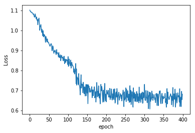
import matplotlib.pyplot as plt
%matplotlib inline
plt.plot(range(epochs*4), losses) #epochs*4 because each epoch is made of 4 batches and for each of them a loss is calculated
plt.ylabel('Loss')
plt.xlabel('epoch');
Saving the Model’s Parameters
torch.save(model.state_dict(), 'IrisDatasetModel.pt')
Only the parameters of the model are saved and not the model itself. For more information on saving and loading visit https://pytorch.org/tutorials/beginner/saving_loading_models.html
Loading a Model
We’ll load a new model object and test it as we had before to make sure it worked.
new_model = Model()
new_model.load_state_dict(torch.load('IrisDatasetModel.pt'))
new_model.eval()
Model(
  (fc1): Linear(in_features=4, out_features=10, bias=True)
  (fc2): Linear(in_features=10, out_features=10, bias=True)
  (out): Linear(in_features=10, out_features=3, bias=True)
)
with torch.no_grad():
    y_val = new_model.forward(X_test)
    loss = criterion(y_val, y_test)
print(f'{loss:.8f}')
0.69291312
References:
- https://pytorch.org/docs/stable/index.html
- https://www.udacity.com/course/deep-learning-pytorch–ud188
- https://stackoverflow.com/questions/49643225/whats-the-difference-between-reshape-and-view-in-pytorch
- https://en.wikipedia.org/wiki/PyTorch
- https://www.analyticsvidhya.com/blog/2018/02/pytorch-tutorial/
- https://www.analyticsvidhya.com/blog/2019/09/introduction-to-pytorch-from-scratch/
![]()