Demystifying Deconvolutions

This article mainly discusses about Up-sampling with Deconvolution. If you’ve heard about the term Deconvolution, and are willing to learn more about it, please read on.

The contents of the this article is as follows:

The need for Up-sampling
Convolution Operation
Going backward
Convolution Matrix
Transposed Convolution Matrix

Deconvolution is also known as Transposed Convolution and Fractionally-strided Convolution.

The need for Up-sampling

When we use neural networks to process or generate images, there is a decrease in the size of the intermediate images in the subsequent layers.

fig1

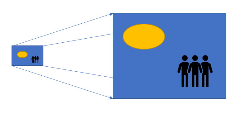
Sometimes, when an output result having the size same as the input image is to be generated, using the learned parameters, up-sampling is useful. This technique is used to up-sample images from low-resolution to high-resolution.

Convolution Operation

I will use a simple example here to discuss about the convolution operation.

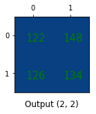
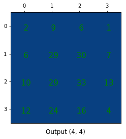
Suppose we have a 4x4 matrix, and we wish to convert it to a smaller 2x2 matrix. This can be accomplished by using a 3x3 “kernel” as shown below.

fig2

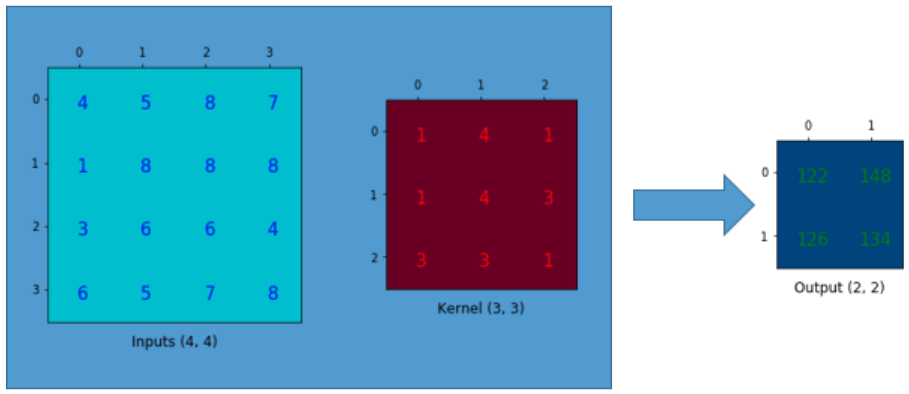
The convolution operation calculates the sum of the element-wise multiplication between the input matrix and kernel matrix. Since we can slide the kernel twice through the input matrix, the resulting output will be of size 2x2.

fig3

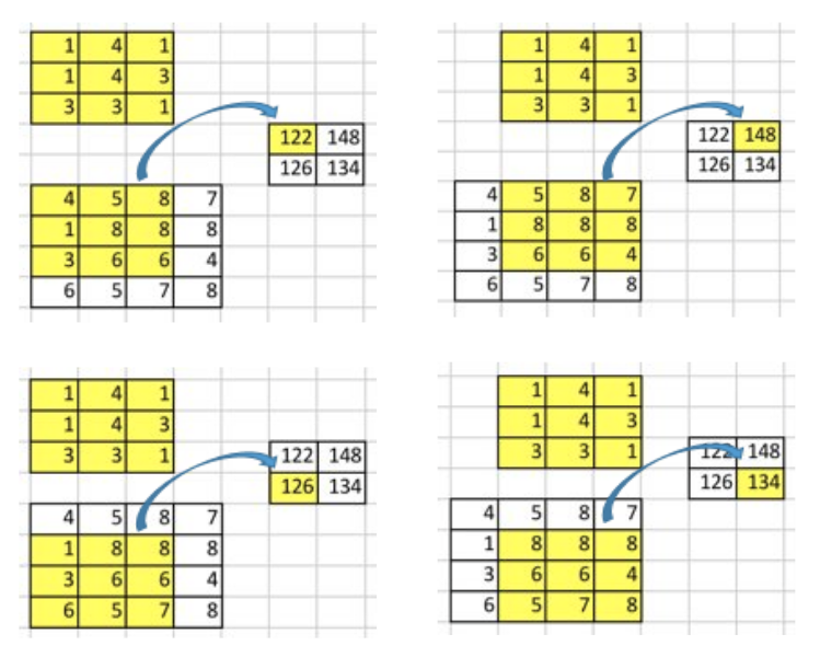
One important point of such convolution operation is that the positional connectivity exists between the input values and the output values.

For example, the top left values in the input matrix (4, 5, 8, 1, 8, 8, 3, 6, 6) affect the top left element in the output matrix (122). This spatial relationship is essential; in images, any set of features on the top-left corner must be showcased in the top-left corner of the resulting smaller image (in the form of learnable parameters).

More concretely, the 3x3 kernel is used to connect the 9 values in the input matrix to 1 value in the output matrix. A convolution operation forms a many-to-one relationship. Let’s keep this in mind as we need it later on.

Going backward

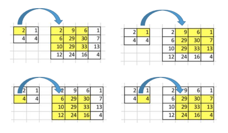
Now, suppose we want to go the other direction. We want to associate 1 value in a matrix to 9 values in another matrix. It’s a one-to-many relationship. This is like going backward of convolution operation, and it is the core idea of transposed convolution.

For example, we could up-sample a 2x2 matrix to a 4x4 matrix, maintaining the 1-to-9 relationship.

fig4

To talk about how such an operation can be performed, we need to understand the convolution matrix and the transposed convolution matrix.

Convolution Matrix

We can view the process of converting a 4x4 matrix to a 2x2 matrix, in another way. We can express a convolution operation using a matrix. It is nothing but a kernel matrix rearranged so that we can use a matrix multiplication to conduct convolution operations.

fig5

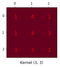
We rearrange the 3x3 kernel into a 4x16 matrix as below:

fig6

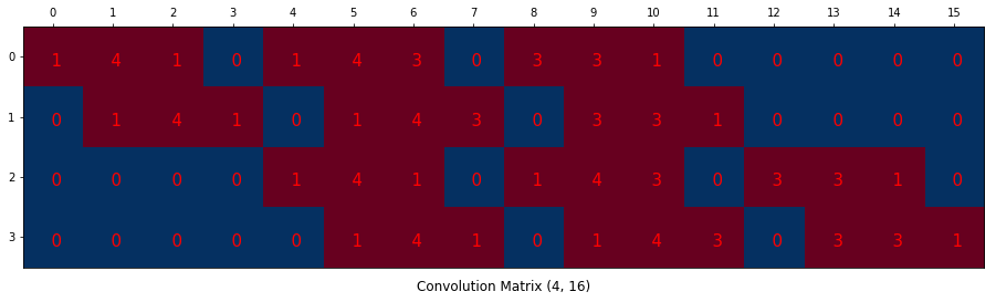
Each row defines a convolution operation, separated by one or more zeros.

The first step is to flatten the input matrix of size 4x4 into a column vector (16x1).

fig7

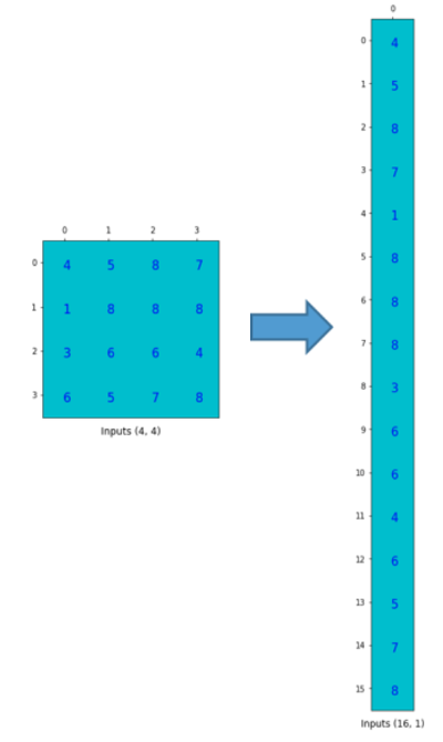
We can matrix-multiply the 4x16 convolution matrix with the 1x16 input matrix (16 dimensional column vector).

fig8

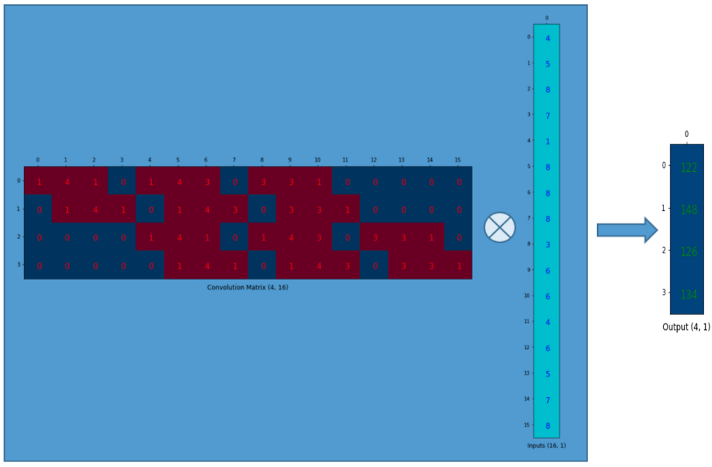
The output 4x1 matrix can be reshaped into a 2x2 matrix which gives us the same result as before.

fig9

In short, a convolution matrix is nothing but rearranged kernel weights, and a convolution operation can be expressed using the convolution matrix.

Transposed Convolution Matrix

We want to go from a smaller 2x2 matrix to a larger 4x4 matrix. But there is one very important thing to consider; we want to maintain the 1-to-9 relationship.

Let us reshape the 2x2 input matrix to a 4x1 column vector as before. If we have a 16x4 matrix with us, we could perform the operation

(16x4) x (4x1) = (16x1)

to get a 16x1 column vector, which we could then resize to the desired 4x4 output.

In order to get this 16x4 matrix, we use the convolution matrix used earlier, whose dimensions were 4x16. If the convolution matrix is denoted by C, then its transpose C^T has the shape (16x4).

Through careful observation, you can convince yourself that the transposed matrix C^T connects 1 value in the input to 9 values in the output.

fig10

The output can be reshaped into 4x4.

fig11

Note: The actual weight values in the matrix does not have to come from the original convolution matrix. They are learnable. What is important is that the weight layout is transposed from that of the convolution matrix (4x16 to 16x4).