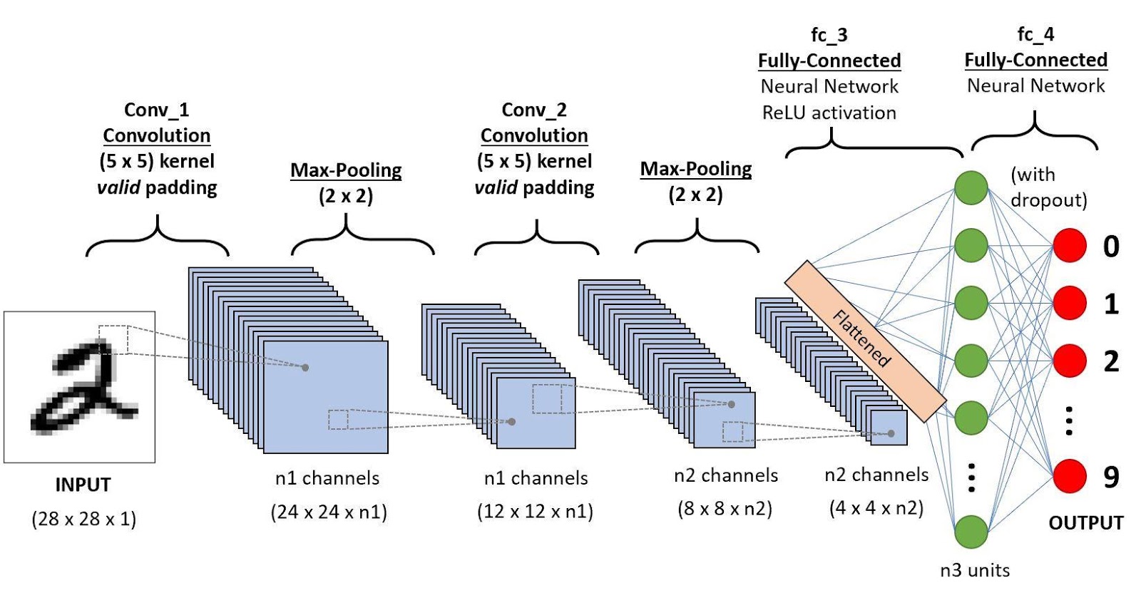
A Convolutional Neural Network is a Deep Learning algorithm which can take an input image, assign learnable weights to various aspects/objects in the image and be able to differentiate one from the other.
It is based on the convolution mathematical operation. Convolution layers consist of a set of filters that are just like two-dimensional matrices of numbers. The filter is then convolved with the input image to produce the output. In each convolution layer, the filter slides across the image to perform the convolution operation. The main agenda of the convolution operation is matrix multiplication of the filter values and pixels of the image, and the resultant values are summed to get the output.
But why ConvNets over traditional neural networks?
Reason 1: Images are Big
Images used for Computer Vision problems nowadays are often 224x224 or larger. Imagine building a neural network to process 224x224 colour images: including the 3 colour channels (RGB) in the image, that comes out to 224 x 224 x 3 = 150,528 input features! A typical hidden layer in such a network might have 1024 nodes, so we'd have to train 150,528 x 1024 = 150+ million weights for the first layer alone. Our network would be huge and nearly impossible to train.
Reason 2: Positions can change
If you trained a network to detect dogs, you'd want it to be able to a detect a dog regardless of where it appears in the image. Imagine training a network that works well on a certain dog image, but then feeding it a slightly shifted version of the same image. The dog would not activate the same neurons, so the network would react completely differently! Moreover, objects in images are made up of small, localized features, like the circular iris of an eye or the square corner of a piece of paper. It seems wasteful for every node in the first hidden layer to look at every pixel.
So let's look at the architecture of a CNN model. It typically comprises of three types of layers
1. Convolutional layers
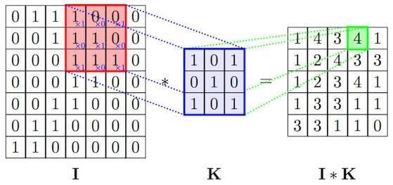
In the convolutional layer, the weight kernel moves to the right with a certain stride value till it parses the complete width. Moving on, it hops down to the beginning (left) of the image with the same stride value and repeats the process until the entire image is traversed.
Conventionally, the first convolutional layer is responsible for capturing the low-level features such as edges, colour, gradient orientation, etc. With added layers, the architecture adapts to the high-level features as well, giving us a network which has the wholesome understanding of images in the dataset, similar to how we would.
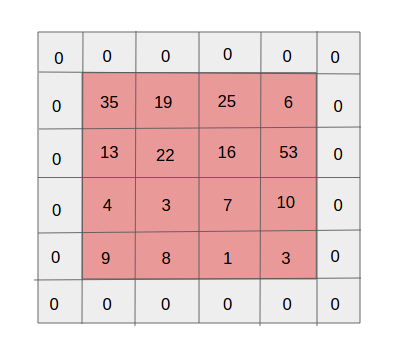
To capture features in the borders, the images are typically augmented with zeros along the four edges. This is known as zero padding.
2. Pooling layers
Just like convolutions, pooling is done to reduce the dimensions of the feature map in order to decrease the computational power required to process the data. The pooled values are further passed into the activation function (sigmoid, ReLU etc.) and input to the next layer.
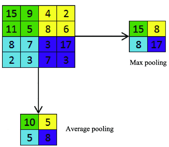
There are two types of pooling, namely Max pooling and Average pooling. In max pooling, the maximum value in a kernel is pooled out whereas in average pooling the mean of the kernel is pooled out for further processing.
3. Fully connected layers
After going through the above processes in multiple layers, the model is able to understand features of various complexity from the training data. Finally, we flatten the final output and feed it to a regular Neural Network for classification.
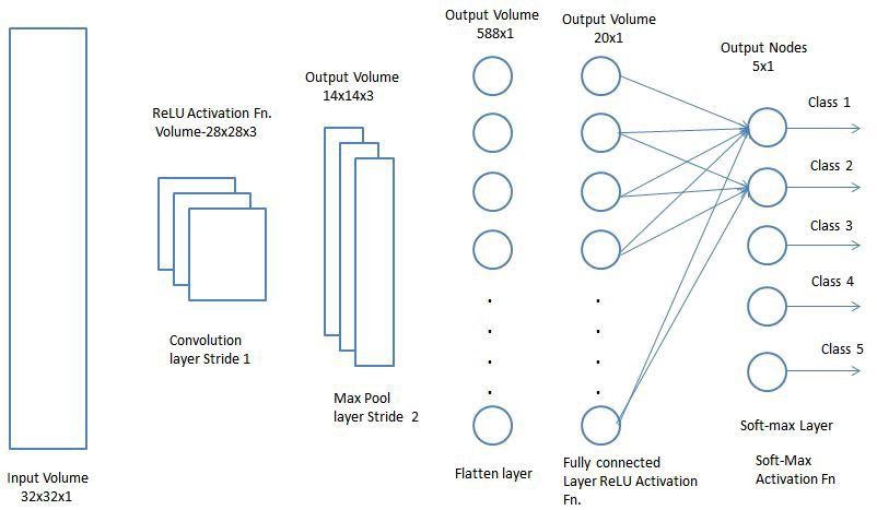
The overall training process can be summarised as follows:
-
We initialize all filters and weights with random values
-
The network takes a training image as input, goes through the forward propagation step (convolution, ReLU and pooling operations along with forward propagation in the Fully Connected layer) and finds the output probabilities for each class.
-
It calculates the total error at the output layer using a loss function like binary cross-entropy, mean-squared error, triplet loss, etc.
-
Finally, it uses backpropagation to calculate the gradients of the error with respect to all weights and uses gradient descent to update them to minimize the output error.The weights are adjusted in proportion to their contribution to the total error.
Now, let's visualize the layers of a ConvNet. Consider the following model taken from one of the sources mentioned below:
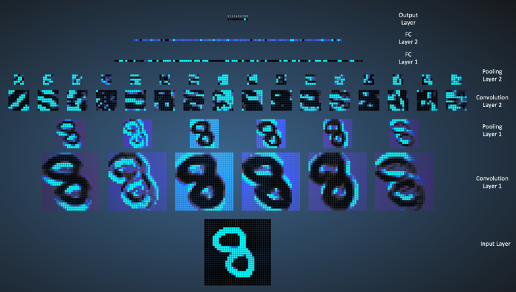
The input image contains 1024 pixels (32 x 32 image) and the first Convolution layer (Convolution Layer 1) is formed by convolution of six unique 5 × 5 filters with stride 1 on the input image.
Convolutional Layer 1 is followed by Pooling Layer 1 that does 2 × 2 max pooling with stride 2 separately over the six feature maps in Convolution Layer 1.

Pooling Layer 1 is followed by sixteen 5 × 5 convolutional filters with stride 1 that perform the convolution operation. This is followed by Pooling Layer 2 that does 2 × 2 max pooling.
Finally, we have the fully connected layers as follows

1)120 neurons in the first fully connected layer
2)100 neurons in the second fully connected layer
3)10 neurons in the third and final fully connected layer. This is the output layer. Note that the pixel corresponding to the digit 8 is the brightest which means the model classifies the hand written digit as 8 with highest probability.
Here are some popular CNN Architectures:
- LeNet-5:

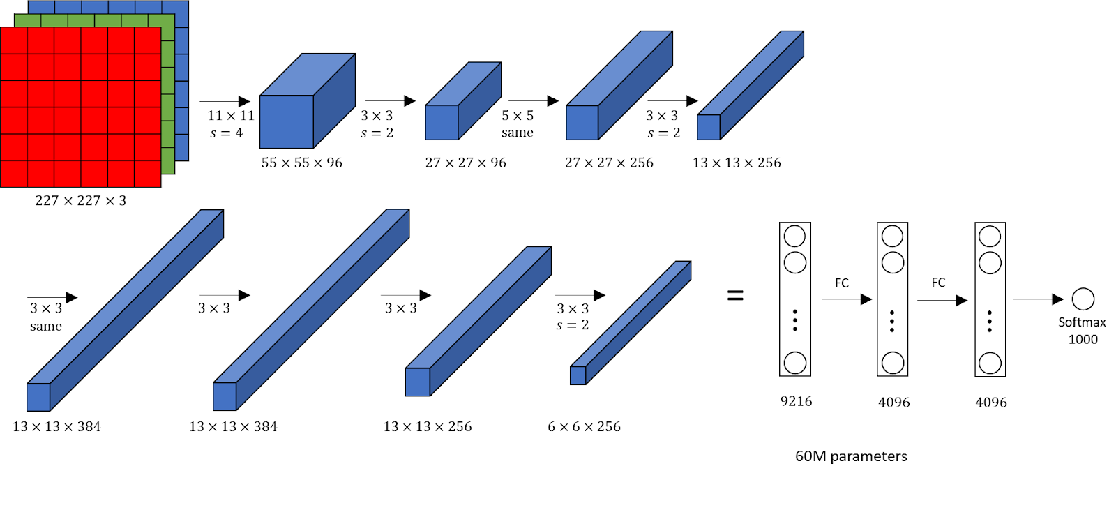
- AlexNet:
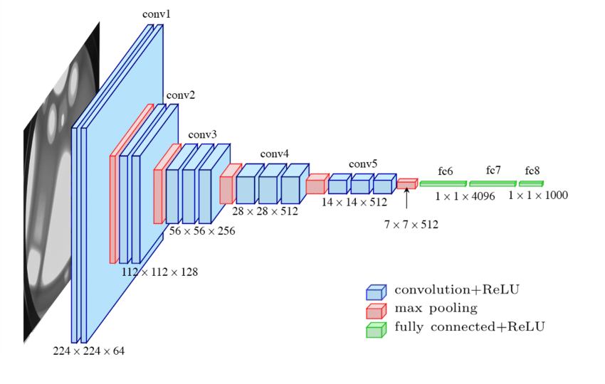
- VGG-16:
Conclusion
ConvNets are a trending topic today in both, academia as well as industry. They are used for a plethora of tasks like object detection and recognition, semantic segmentation, medical imaging and many more.
In this blog, I have tried to explain the fundamental concepts of convolutional neural networks with substantial simplicity. We have seen the types of layers used in ConvNets, some popular CNN architectures and visualized different layers from a model. Hope it was informative!
References:
https://www.analyticsvidhya.com/blog/2018/12/guide-convolutional-neural-network-cnn/
https://ujjwalkarn.me/2016/08/11/intuitive-explanation-convnets/
