An intuition on how RNN and LSTM works

An intuition on how Recurrent Neural Networks and LSTM works

Let us first try to understand how RNNs work and how they are used to solve sequence modeling tasks that require the model to store the information seen before.

Working of RNN

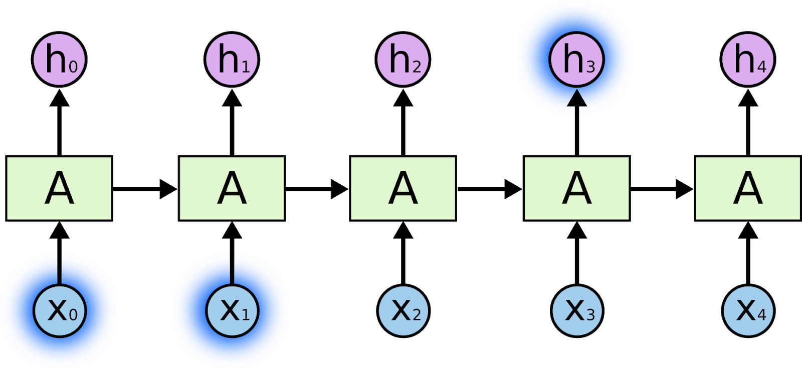
At time step 0, RNN takes the input X₀, predicts an output h₀, and stores the information in the state S₀. Now, for the next time step, the RNN takes the current input X₁ along with the information from the previous state S₀ and predicts the output h₁ subsequently storing the information from the previous state and the input in S₁. This process continues until time T.

You can notice that at some time step t, state S_t carries all the information seen until then.

Analogy between RNN and a whiteboard

Now let us try to draw an analogy between RNN and a whiteboard.

Let us say we want to do some calculation on a whiteboard, which has limited space. At periodic intervals, we see all the information that we have written on the board until then and then figure out the next step and write some more information on to the board.

We can notice that after some time, we are bound to overwrite the previous information that we wrote because of the limited space of the board.

Now at some time step t, we would have written so much that there would be no way for us to know what we had written at timestep t - k and we also wouldn’t be able to find how much error was caused due to whatever we calculated at timestep t - k.

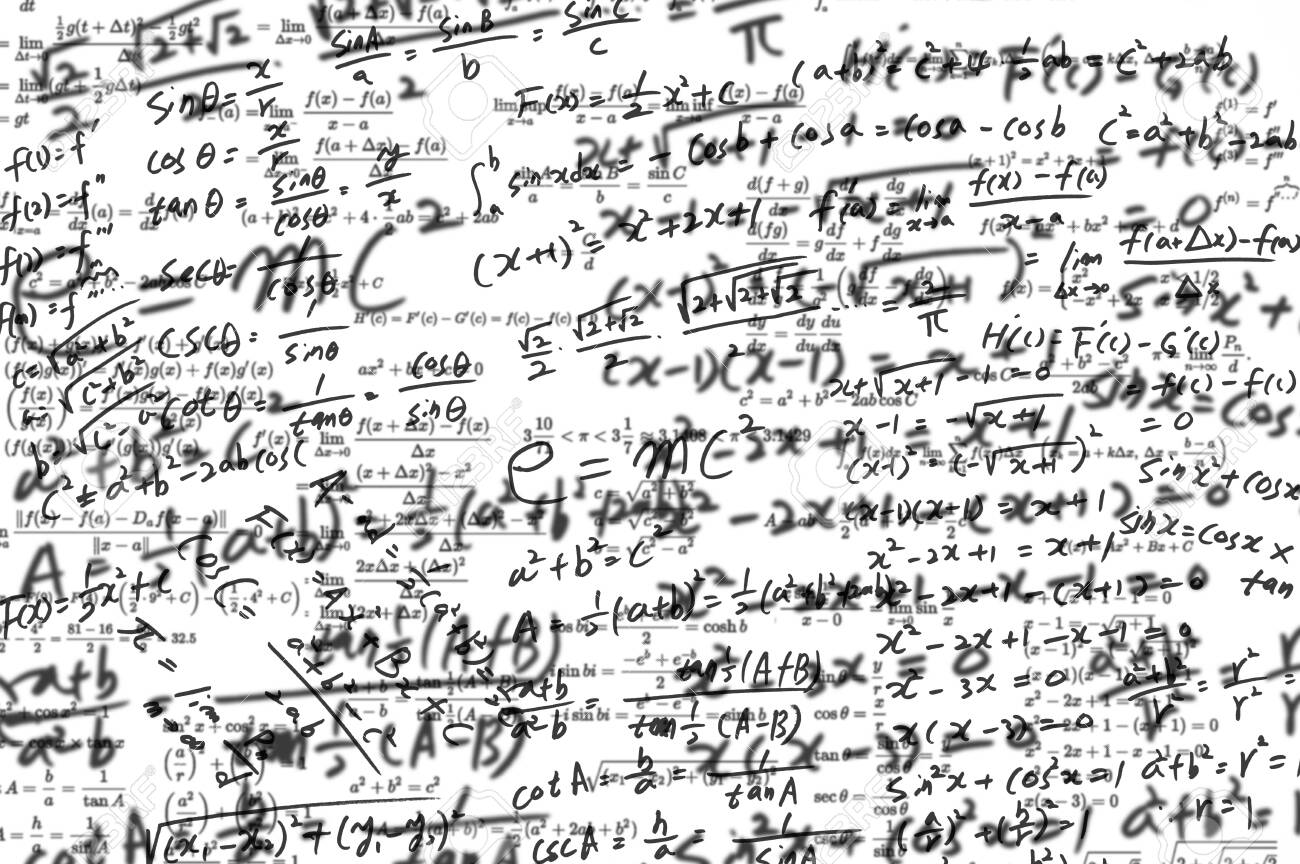
We can see how the state S_t in RNN is similar to a whiteboard with all the information cramped to limited space and how calculating S_t+1 from S_t and the input is similar to writing more information on the filled board.

This gives us intuition about why RNN fails to perform well when there are strong dependencies on information seen long before.

For example, if we had a sentence,
Alice lives in France. She is an artist. She likes to cook. She speaks
and had to predict the next word, we could easily say that it would be French but it would be difficult for the RNN model to remember the word France seen long before and hence fails to predict the correct next word.

Math behind RNN

Let us now see the actual math that goes behind RNN.

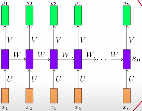
At a time step t, State S_t and output y_t is given by, where U, V and W are the parameter weights, b is the the bias, X_t is the current input, S_t-1 is the previous state,c is the bias, S_t is the current state and sigma is the sigmoid function of x.

Solving efficiently on a whiteboard

Let us now try to see how we can solve the whiteboard problem to build an intuition about LSTM.

Let us take a scenario where we have to evaluate the expression,

on the whiteboard but the whiteboard has space to accommodate only 2-3 steps.

Now instead of writing something like, 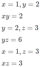We could just write,

Let us call this selective writing where we are writing only specific information instead of writing everything on to the board.

Now, while reading from the board to make the next step, we only need the information about xy and xz but not yz for the next step. So, we can only read whatever is important for the immediate timesteps and we will call this selective reading.

After plugging in the values on the board, we get, We can see that we don’t need the xy or xz values anymore and we can erase them from the board instead of keeping everything on the board like before. We are essentially forgetting specific information that we think is not relevant anymore. We will call this step selective forgetting.

We saw that by using selective read, write, and forget instead of blindly writing and keeping everything, we can solve the whiteboard problem to an extent.

Analogy between LSTM and the whiteboard

Let us now see how LSTM is similar to this technique.

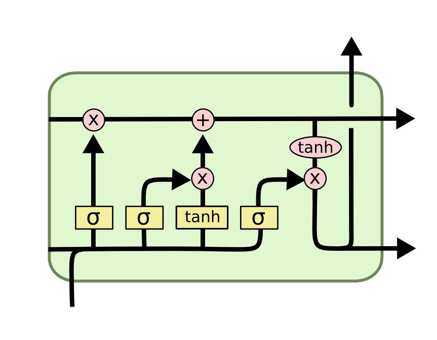
While passing the information of the previous state S_t-1 to the next state, we don’t pass the whole information like RNN, instead, we introduce a gate and specify how much percent of each value should be passed similar to the selective writing on the board.

After taking in information from the previous state and the current input to calculate the current state, we introduce one gate to specify how much should be read from this state similar to selective reading.

Finally, instead of keeping all this information in the current state, we introduce one more gate which specifies how much percent of each value should be kept in the state and how much should be discarded similar to the selective forget that we saw above.

If the same example,
Alice lives in France. She is an artist. She likes to cook. She speaks
is given to the LSTM model to predict the next word, it would retain the information France seen long before using gates and would be able to predict the next word as French.

Math behind LSTM

We will now see the mathematical equations behind LSTM,

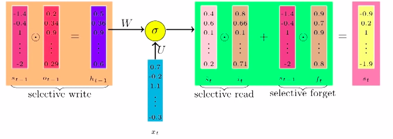The previous state S_t-1 is passed through an output gate o_t-1 to get the state h_t-1. These are given by,

An intermediate state is then found from the current input X_t and the previous state h_t-1 which is then passed through the input gate i_t

The final state S_t is then found after applying input gate and forget gate f_t respectively as,

Conclusion

Thus we intuitively understand the architecture of LSTMs and RNNs and then connect it with the actual mathematical equations that go behind these models. We also get an intuitive understanding of why LSTM has a better architecture, and how it helps them in performing better than RNN, and solve the problems like long-term dependencies in RNN to an extent.

References

1. Deep Learning NPTEL course
2. LSTM colah’s blog
3. LSTM tutorial