Solving a traffic problem using graph decomposition

The Capital city is known for its prosperous life and big opportunities. Its inhabitants are called “capitolates”. Every capitolate in Capital city wants to live a happy and peaceful life. Now Capital city has three divisions - Residential town, Fun town and market city. Residential town is where capitolates live. Fun town is where they meet friends and make merry. Market city is where they work to make a living. But every passing year, capitolates are becoming more and more frustrated and unhappy. The reason is that people from neighbouring lands want to become capitolates and are moving to Capital city. This is making the roads busier and traffic slower. In particular, every road intersection in market city has become a deadly traffic bottleneck.

The ten peace-keepers of Capital city propose an unconventional solution to this traffic problem - “Transform market city and make all the roads one-way”. But at this juncture a few questions arise:

1. In what direction should each one-way road go?

2. Is every traffic intersection in market city still reachable from every other traffic intersection in market city using these one-way roads? If not, which intersections are not reachable from one another?

Now, the nine hard working peace-keepers explore different possible one-way transformations of market city. They call the transformation “good” if every traffic intersection is reachable from every other traffic intersection. They assign the tenth peace-keeper, the lazy one, the job of finding whether a given transformation is “good”. If you are the tenth peace-keeper, you are in luck, for we will show you how to accomplish this task, in a fraction of a second, using our vast computing power.

Formal ideas and definitions

Before we present a solution to our main problem, we first define some mathematical terms and explore a few key ideas. We will then redefine the main problem statement using those mathematical terms. We will explore the following ideas.

• The idea of a graph

• Exploring a graph

• DFS (Depth First Search)

• Connectedness and connected components of a graph

• Directed graphs

• Strong connectedness

The idea of a graph

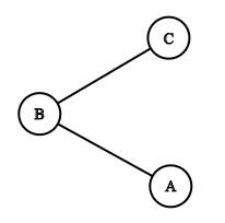
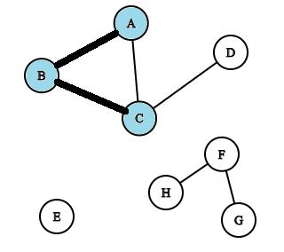
In mathematics, and graph theory, a graph is a set of objects in which some pairs of the objects are in some sense “related”. The objects are called vertices(also called nodes) and each of the related pairs of vertices is called an edge. In the picture, A, B and C are the vertices and the pairs (A, B) and (B, C) are edges.

Many important phenomena can be represented using graphs. Examples are:

• Webpages connected by links

• Intersections connected by roads

• People connected by friendships in social networking.

Formally, a graph G is a collection v of vertices, and a collection E of edges, each of which connects a pair of vertices.

Exploring a graph

We have the following definition for a path in G:

A path in a graph G is a sequence of vertices v₀, v₁, v₂, …, v_n so that for all i, (v_i, v_i+1) is an edge of G.

We now have a tool to define Reachability:

Two vertices u and v (u not equal to v) are reachable if there exists a path from u to v.

When we say we explore a graph G, it means that we start at an “unvisited” vertex v of the graph and then start visiting vertices that are reachable from v using the edges in G. Once we finish visiting all vertices reachable from v, we mark the visited vertices as “visited”. Initially, all vertices are “unvisited”.

Depth First Search (DFS)

The next thing we will do is give a way to reach all vertices of a graph. The idea is intuitive and easy to understand. What DFS does is, it starts at an unvisited vertex of G and explores it, and continues to do this for every other unvisited vertex of G. So when DFS finishes, we end up visiting every vertex of G.

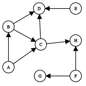
For example, consider the following graph on eight vertices.

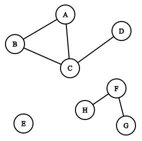
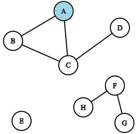
When we run DFS on the graph, we start at some vertex of the graph, say, A. We then explore A:

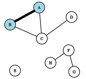
A is visited

B is visited

C is visited

D is visited

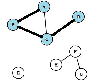
After exploring A as shown in the pictures, we check for other unvisited vertices. Since B, C, and D are already visited, our next unvisited vertex is E. We explore E, and then, F. After exploring F, we will have visited all vertices. This completes our DFS exploration.

Connectedness

Connectedness in a graph G is a property which helps us understand which vertices in G are reachable from which others. The following theorem holds for every graph G:

The vertices of G can be partitioned into Connected Components so that a vertex v is reachable from a vertex w if and only if they are in the same connected component.

In the graph above, the vertices {A, B, C, D} form the first connected component. The vertex {E} forms the second connected component. Finally the vertices {F, G, H} forms the third connected component.

You might realize that this notion of connectivity gets us closer to the problem that we want to solve. But we are not quite there yet. We also have to tackle the issue of one-way roads. Before we move on, we give a modification of the DFS algorithm to give ourselves more capability. We introduce a new feature - pre and post orderings. We store two variable called previsit and postvisit for every vertex. Every vertex is given the label (previsit/postvisit).

We store an extra variable called clock. Each time we enter or leave a vertex the value of the clock is incremented by 1. We assign pre and post order values to each vertex as follows:

1. During exploration, each time a vertex v of the graph is visited, we assign the current value of clock to the previsit value of v.

2. When exploration of v finishes, we assign the new value of the clock to the postvisit value of v.

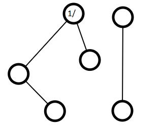
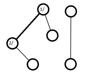
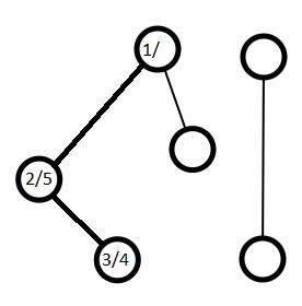
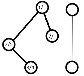
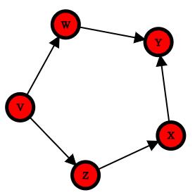
Example: Consider a graph on six vertices.

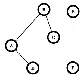
The following illustration shows how previsit and postvisit values are assigned to the vertices when we run DFS on the graph.

Clock = 1:

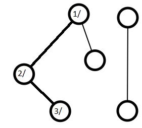
Clock = 2:

Clock = 3:

Clock = 4:

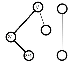
Clock = 5:

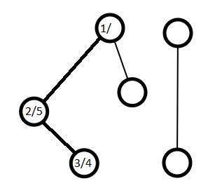
Clock = 6:

Clock = 7:

Clock = 8:

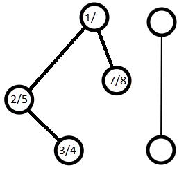
Clock = 9:

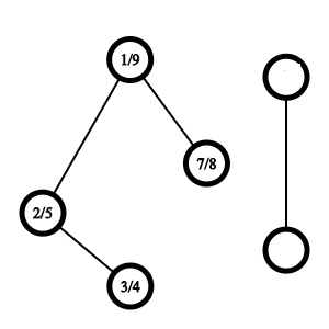
The other component of the graph is given pre and post orderings in a similar fashion. After all components are assigned pre/postvisit numbers, the graph looks like:

Directed Graphs(DiGraphs)

A directed graph is a graph where each edge has a start vertex and an end vertex.

Examples are:

• Streets with one-way roads (an abstraction of our traffic problem)

• Links between webpages.

• Followers on social networks like instagram

• Dependencies between tasks (sometimes some tasks need to be performed before others).

Strong Connectedness

Strong connectedness in a directed graph is analogous to connectedness in a non-directed graph.

For any two vertices in a digraph v and w, there are three different possibilities:

1. w is reachable from v and v is reachable from w.

2. Exactly one of v or w is reachable from the other.

3. w is not reachable from v and v is not reachable from ww.

The first case sets up the basis for strong connectedness.

A directed graph can be partitioned into strongly connected components (SCCs) where two vertices are connected if and only if they are in the same component.

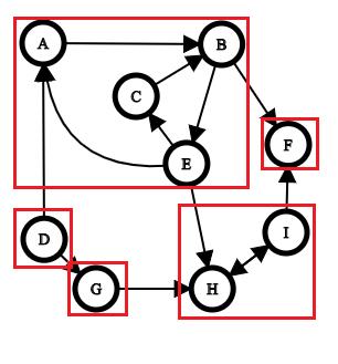
Consider the graph P below:

The sets { A, B, C, E }, { H, I }, {D}, {F}$ and {G} form the five strongly components of the above graph P.

We define the final tool that we will use to solve our problem:

The metagraph M of a directed graph G is the graph with its vertex set as the set of SCCs of G and edges showing how the SCCs connect to each other.

It should be noted that the metagraph of G will be a Directed Acyclic Graph (A directed graph with no cycles) or a DAG. This property should hold, since if there were a cycle in M, then we will have at least two SCCs in G, which are a part of the cycle, reachable from each other, which contradicts the fact that they belong to two different SCCs.

The graph below is the metagraph of the graph P we have described in the above picture.

In the above metagraph, W is the SCC consisting of the vertices A, B, C and E, Y is the SCC consisting of the vertex F, X is the SCC consisting of the vertices H and I, Z is the SCC consisting of the vertex G and V is the SCC consisting of the vertex D.

We now have the tools to simplify our main traffic problem. Market city can be seen as a DiGraph with the one-way roads as edges. We just have to compute the strongly connected components of market city.

The algorithm we use to get our work done here is called Kosaraju’s algorithm.

An abstraction of the problem

Given a DiGraph G, compute the strongly connected components of G.

This is a simpler version of our original problem.

Naively, what we can do is, for each vertex v in G, we can explore v to find the vertices that are reachable from v. And then, we can find the vertices u reachable from v that can also reach v. This, by definition, will give us the strongly connected components of G. But the problem with this procedure is that it takes a lot of steps to complete. We want to design a much faster algorithm. To achieve that, we make a few elegant observations.

1. Sink SCCs: An important theorem in graph theory tells us that for a DAG, there always exists a sink vertex (a vertex with no outgoing edges) and a source vertex (a vertex with no incoming edges) in the DAG (We leave the proof as an exercise). For our problem, the DAG in question is the metagraph M. Hence, there is a “sink strongly connected component(sink SCC)” in G.

The idea is that if a vertex v is in a sink SCC, then if we run explore on v, we will find all the vertices in the strongly connected component that v is in.

But we need a way to find a sink SCC of G.

1. Another important theorem in graph theory tells us that in a DAG, the vertex with the largest postvisit number lies in a source vertex of the DAG (Proof can be found here). Again, the DAG in question is the metagraph M. Hence, the vertex with the largest postvisit number in G lies in a source SCC of G.

2. Our problem was that we wanted a sink component. But we know how to find a source component. So we reverse the direction of all the edges in G to find the transpose of the graph G^R. The following properties hold for G^R:

• G^R and G have the same SCCs.

• Source components of G^R are sink components of G^R.

• The vertex with the largest postorder in G^R is in a sink SCC of G.

We are in the home stretch now. Our job is much simpler. We just run DFS on G^R and assign pre/postvisit numbers to every vertex. Then we start removing the components associated with the vertex with the largest postvisit number in G^R. In the end, we end up finding the SCCs of G. We illustrate the procedure on the sample graph we described before.

G:

G^R:

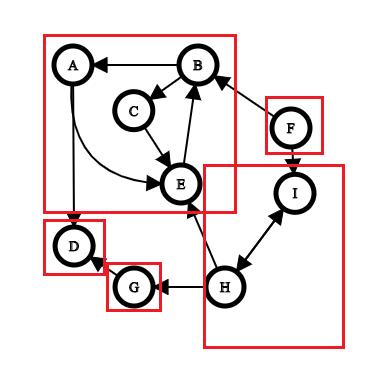
We first assign pre and post visit numbers to every vertex:

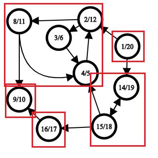
We remove the SCC with the vertex with the highest post order number. That is we first remove the vertex F and all the edges going from F:

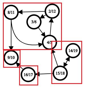
From the resulting graph above, we remove the component having the vertex with the next highest post visit number, that is I:

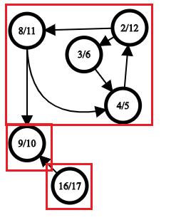
We continue this process until we have found all the SCCs:

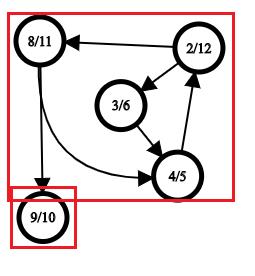
And finally:

The algorithm we explained now is called Kosaraju’s Algorithm. This completes the solution to our problem. The transformation is good if there is only one strongly connected component. We have successfully found out the disconnected intersections in market city!

A mathematical analysis of the above algorithm shows that the total time it takes to run the algorithm is proportional to the sum of the total number of vertices and the total number of edges in the graph. Today’s computers can accomplish this within the blink of an eye!