Machine Learning is broadly classified into three main categories -
- Supervised Learning - used when all the available data is annotated
- Unsupervised Learning - no annotated data is available
- Semi Supervised Learning.
Supervised Learning includes models like linear regression, whereas unsupervised has logistic regression. Semi-supervised Learning falls between unsupervised Learning (with no labelled training data) and supervised Learning (with only labelled training data). It is a remarkable instance of weak supervision.
Semi Supervised Learning (SSL) is an upcoming field that is gaining popularity day by day. It is an approach to machine learning that combines a small amount of labelled data with a large amount of unlabeled data during training. When labelled data isn’t available due to various reasons, unlabeled data when used in conjunction with a small amount of labelled data can produce considerable improvement in training accuracy. The collection of labelled data for a learning problem often requires a skilled human agent or a physical experiment. Since the cost of acquiring labelled data is very high, it renders these training sets infeasible, whereas the collection of unlabeled data is relatively inexpensive. The best example of this is medical images such as X-Rays. Getting labelled X-ray images involves a lot of time to be spent by the doctors which isn’t feasible. In such situations, semi-supervised Learning can be of great practical value. Semi-supervised Learning is also of theoretical interest in machine learning and as a human learning model.
A Semi-Supervised algorithm assumes the following about the data:
- Continuity Assumption: The algorithm assumes that the points which are closer to each other are more likely to have the same output label.
- Cluster Assumption: The data can be divided into discrete clusters and points in the same group are more likely to share an output label.
- Manifold Assumption: The data lie approximately on a manifold of a much lower dimension than the input space. This assumption allows the use of distances and densities which are defined on a manifold.
The basic working of an SSL model is as given:
- Train the model with the small amount of labelled training data just like you would in supervised Learning until it gives you good results.
- Then use it with the unlabeled training dataset to predict the outputs, which are pseudo labels since they may not be entirely accurate.
- Link the labels from the labelled training data with the pseudo labels created in the previous step.
- Link the data inputs in the labelled training data with the inputs in the unlabeled data.
- Then, train the model the same way you did with the labelled set in the beginning in order to decrease the error and improve the model’s accuracy.
The above method is commonly known as the self training method or psuedo label method. However, this method becomes heavily dataset dependent and in some cases might reduce accuracy by a great extent.
The algorithm for psuedo label is as follows:
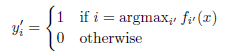
Pseudo-Label are target classes for unlabeled data as if they were true labels. The class, which has maximum predicted probability predicted using a network for each unlabeled sample, is picked up:
Pseudo-Label is used in a fine-tuning phase with Dropout. The pre-trained network is trained in a supervised fashion with labeled and unlabeled data simultaneously:
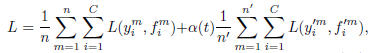
where n is the number of samples in labeled data for SGD, n’ is the number of samples in unlabeled data; C is the number of classes; fmi is the output for labeled data, ymi is the corresponding label; f’mi for unlabeled data, y’mi is the corresponding pseudo-label;
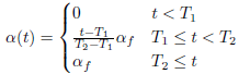
α(t) is a coefficient balancing them at epoch t. If α(t) is too high, it disturbs training even for labeled data. Whereas if α(t) is too small, we cannot use benefit from unlabeled data.
α(t) is slowly increased, to help the optimization process to avoid poor local minima:
One more popular algorithm used for SSL is known as the TMean Teacher Model
In the mean teacher model, two identical models are trained with two different strategies called the student and teacher model. In which, only the student model is trained. And, a very minimal amount of weights of student model is assigned to the teacher model at every step called exponential moving average weights that’s why we call it as Mean teacher.
There are two cost functions to be calculated here which is important during back propogation. The cost functions are:
- Classification cost(C(θ)) - binary cross-entropy between label predicted by student model and original label.
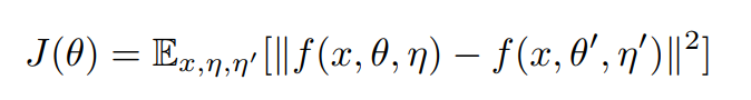
- Consistency Cost(J(θ)) - mean squared difference between the predicted outputs of the student (weights θ and noise η) and teacher model (weights θ′ and noise η′).

Consistency cost is actually the distribution difference between two predictions (student and teacher prediction) and the original label is not required. During training, the model tries to minimize the distribution difference between the student and teacher model. So, instead of labeled data, we may utilize unlabelled data here. The mathematical declaration of consistency cost is as follows.
While back-propagating in the student model, the overall cost (O(θ)) is calculated with the given formula:
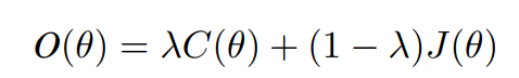
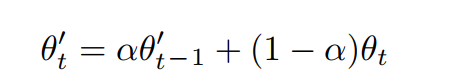
During training, the exponential moving average(EMA) weights of the student model are assigned to the teacher model at every step and the proportion of weights assigned is controlled by parameter alpha(α). As mentioned in equation 3, while assigning weights, the teacher model holds its previous weights in alpha(α) proportion and (1−α) portion of student weights.
With the amount of data growing exponentially, there is no time to label and annotate them. This is where semi supervised learning comes into the picture. SSL is used in various aspects of our lives nowadays. Its most common practical uses include Speech Analysis, Web Content Classification, Protein Sequence Classification, Text Document Classifier, etc.
References