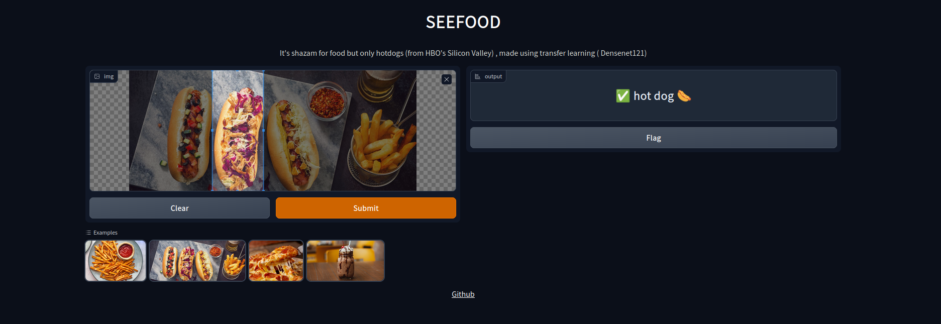
SEEFOOD is an application which basically predicts if an image is an image of a hot-dog or not. This is based on the model used in the HBO’s Silicon Valley .

This blog is a short tutorial on building this classfier model. Knowing the basics of Deep Learning, CNNs and Transfer learning would be helpful in following along.
How to start ?
First, we need to get a dataset for training the model. For this, there is a dataset on kaggle which perfectly matches our needs. So now that we have a dataset, we need to build and train the actual model.
Let’s start coding.
The notebook is here if you want to follow through as you’re reading the article.
First, off we import all the required libraries.
import torch
from torchvision import datasets,transforms, models
from torch import optim , nn
from torch.utils.data import DataLoader
import torch.nn.functional as F
import matplotlib.pyplot as plt
Before importing the dataset we can use a simple transform to ensure all our images and resized, center cropped, and convert into tensors.
transforms = transforms.Compose([transforms.Resize(256),
                                 transforms.CenterCrop(224),
                                 transforms.ToTensor(),])

dataset = datasets.ImageFolder(root='gdrive/My Drive/seefood/train/',transform=transforms)
validation_set = datasets.ImageFolder(root='gdrive/My Drive/seefood/test/',transform=transforms)
Now we can import both the test and validation sets. Since the number of images here is not very high we can use a batch size of 20.
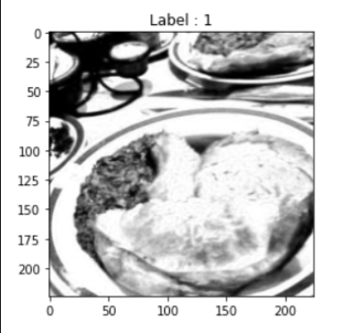
Once the dataset is loaded we can view the images.
trainLoader = DataLoader(dataset, batch_size=20,shuffle= True)
valLoader = DataLoader(validation_set,batch_size=20,shuffle=True )

data = iter(trainLoader)
images ,labels = next(data)
plt.imshow(images[0][0,:,:],cmap='gray')
plt.title(f"Label : {labels[0]}")
Building the model
Since we are dealing with images we would need to use a model which is based on Convolutional Neural Networks (CNNs). The model itself would be a binary classifier to detect whether the food item is a “hot dog” or not. Smaller models with lower layers do not tend to work because they are simply not powerful enough to detect the different features, so we can see a good use case of transfer learning here.
For this purpose we can use the densenet121 model, you can read more about Densely Connected Convolutional Networks in this paper here. . Since we are only going to train the last block of the model we can freeze all the other parameters of the model.
model = models.densenet121(pretrained=True)
for params in model.parameters():
  params.require_grad = False
#model.classifier -> Linear(in_features=1024, out_features=1000, bias=True)
If we take a look at the classifier currently we can see it’s a classifier that has 1024 input features and 1000 output features. We can redefine this classifier for our case here.
classifier = nn.Sequential(nn.Linear(1024,1024),nn.ReLU(),nn.Dropout(p=0.3),
                           nn.Linear(1024,512),nn.ReLU(),nn.Dropout(p=0.3),
                           nn.Linear(512,2),nn.LogSoftmax(dim=1))
model.classifier = classifier
The classifier now,
model.classifier -> Sequential(
  (0): Linear(in_features=1024, out_features=1024, bias=True)
  (1): ReLU()
  (2): Dropout(p=0.3, inplace=False)
  (3): Linear(in_features=1024, out_features=512, bias=True)
  (4): ReLU()
  (5): Dropout(p=0.3, inplace=False)
  (6): Linear(in_features=512, out_features=2, bias=True)
  (7): LogSoftmax(dim=1)
)
Training the model
For the loss function here we can use the negative log-likelihood loss. Since we are training only the classifier part of the model, we need to include only the parameters from that block in the optimizer.
loss_function = nn.NLLLoss()
optimizer = optim.Adam(model.classifier.parameters(), lr=0.003)
If you are trying to train the model, do make use of GPUs on google colab or kaggle. This speeds up the training process a lot. The standard training loop,
loss_graph , val_loss_graph , acc = [] , [] , []
for _ in range(6):
  running_loss = 0
  val_loss = 0
  device = torch.device("cuda" if torch.cuda.is_available() else "cpu")
  model.train()

  for images, labels in trainLoader:

    images , labels = images.to(device), labels.to(device)
    optimizer.zero_grad()
    logits = model(images)
    loss = loss_function(logits,labels )
    running_loss += loss.item()
    loss.backward()

    optimizer.step()

  with torch.no_grad():
    model.eval()
    cor = 0
    total = 0

    for images,labels in valLoader:
      images , labels = images.to(device), labels.to(device)
      predictions = model(images)
      loss = loss_function(predictions, labels)
      val_loss += loss.item()

      for p,l in zip(torch.argmax(predictions,dim=1 ),labels):
        if p==l:
          cor +=1
        total +=1

  loss_graph.append(running_loss/len(trainLoader))
  val_loss_graph.append(val_loss/len(valLoader))
  acc.append(cor*100/total)
  print(f'training loss : {running_loss/len(trainLoader)} , validation loss : {val_loss/len(valLoader)} , Accuracy : {cor*100/total}')
training loss : 0.8344280552864075 , validation loss : 0.38366479575634005 , Accuracy : 87.4
training loss : 0.3701903349161148 , validation loss : 0.4923225581645966 , Accuracy : 76.2
training loss : 0.40178473711013796 , validation loss : 0.26429639220237733 , Accuracy : 90.2
training loss : 0.29359916508197786 , validation loss : 0.2639751332998276 , Accuracy : 89.6
training loss : 0.23448901653289794 , validation loss : 0.26386004567146304 , Accuracy : 89.6
Result
On training it for about 6 epochs I got around 86% accuracy. You can try this here

Interesting question ?
Why do you think densenet121 was used for this model ?
Links and resources