Long Short Term Memory Neural Networks or LSTM Neural Network is a commonly used Recurrent Neural Network model that is most commonly used in tasks like speech recognition, music generation etc. Lets take a deep dive into what Recurrent Neural Networks are and why we need and use LSTMs.

Long Short Term Memory Neural Networks

Recurrent Neural Networks and Why LSTMs?

Recurrent Neural Networks are those Neural Networks that we use to process information that require us to keep informed of previous information. In simpler words, when we want a model to perform a certain category of tasks like speech recognition, music generation, machine translation, sentiment classification, etc, all of which invloves keeping track of previous information (like keeping track of all the words while processing a sentence during machine translation), a normal Neural Network cannot do this, while a Recurrent Neural Network, which keeps a track of the past information in it’s internal state addresses this issue.

Recurrent Neural Network - Unrolled

The above diagram is that of a basic Recurrent Neural Network, the chained structure is appropriate for modeling sequences and using this structure for Neural Networks have proven to work for the above mentioned applications. LSTMs come into play when a certain problem occurs within RNNs itself.

Problem of Vanishing Gradients due to Long Term Dependencies

Consider the following small sentence: She was riding her cycle . Predicting the word ‘her’ using RNNs is relatively easy since it just has to process the immediate words next to it, but predicting some sort of information that requires some sort of context from earlier, for example, mentioning I am from France in the beginning of a paragraph, but having to predict the language that was spoken much later in the text. Here, as the gap between relevant information grows, it becomes difficult for RNNs to connect both information to make a valid prediction. This happens because while calculating gradients for the weights during backpropagation, the values from one end of the sequence may find it difficult to influence that in other ends of the sequence which may or may not play an important role in prediction. This is the case in normal RNNs, where ‘long range dependencies’ are not really supported.

This is where LSTMs come into play!

Long Short Term Memory Networks

Long Short Term Memory Networks (usually just called LSTMs) are a special kind of RNN, capable of learning long-term dependencies. They were introduced by Hochreiter & Schmidhuber (1997). They are explicitly designed to avoid the long-term dependency problem by remembering information for long periods of time, and this is possible by introducing ‘memory cells’ which keep track of these dependencies throughout the sequence.

Long Short Term Memory Network

This is how an LSTM looks like, it follows the same chain like structure like that of the RNNs, but it contains several added gates. It may seem difficult to process this as a whole, but we’ll walk through this step by step.

Note: The sigmoid function returns a value between 0 to 1 and this case, values very close to either 0 or 1 and hence is commonly used in our gates to make a particular decision.

The following are states and gates involved in an LSTM cell:

1. Activation layer: This layer consists of the activation values like the normal RNNs do
2. Memory Cell or Candidate layer: This layer is involved in keeping track of dependencies
3. Update Gate: Sigmoid function that decides whether or not the memory cell should keep track of the dependecy
4. Forget Gate: Sigmoid function that decides whether or not the memory cell should leave or forget the dependency
5. Output Gate: Sigmoid function that helps us filter what parts of the memory cell layer we want to pass into the output

LSTM Structure Inside

If the diagram is overwhelming, the following equations may help you to walk through the process.

This is the calculation for a memory cell initially which takes into account the previous activation layer and input layers’ weights, and adds it to a bias, while passing the resultant to a tanh function that returns a score between -1 and 1, which in turn carries a dependency.

Here, the decision is made whether or not to keep track of the dependency with the help of the update and forget gates, which are sigmoid layers.

Here, we decide what exactly to update into the memory cell, which either retains the dependency from earlier or updates it to a new value based on the decision made by the update and forget gates. Hence, the output will be filtered. This is done by running a sigmoid function layer to decide which parts of the memory cell we will send to the output and while the memory cells will be passed through tanh and then passed through the output gate to get only the filtered output. Here, our memory cells are updated appropriately.

The activation layer is influenced by certain memory cell values decided upon by the output gate, and is appropriately updated and passed onto the next cell.

The resultant \(\hat{y}^{<t>}\) vector is obtained by passing the activation layer through a softmax function, but do note that this step is dependent on what problem we’re solving and isn’t part of the general LSTM framework.

Character to Character LSTM Model

We are going to use a two layer LSTM model with 512 hidden nodes in each layer. We will make the model read a text file that contains text from a transcript, in this example we will make the model read an exerpt from ‘The Outcasts’, we will then use the same sequence but shifted by one character as a target.

Before we get started, here are some key terms to get used to:

1. Vocabulary: This is a set of every character that our model requires
2. LSTM Cell : We will make use of pyTorch’s LSTM cell that has the structure, as explained earlier
3. Hidden State or Activation State: This is a vector of size(batch_size, hidden_size), the bigger dimension of the hidden_size, the more robust our model becomes but at the expense of computational cost. This vector acts as our short-term memory and is updated by the input at the time step t.
4. Layers of an LSTM: We can stack LSTM cells on top of each other to obtain a layered LSTM model. This is done by passing the output of the first LSTM cell from the input to the second LSTM cell at any given time t, this gives a deeper network.

The code with explanation in comments is provided at the references section of this article

The model receives an “A” initially as an input to the LSTM cell at time t=0. After that, we get the output with the size of our vocabulary from the memory cell. If we apply softmax function to the output, we get the probabilities of the characters. Then we take ‘k’ most probable characters and then sample one character according to their probability in the space of these ‘k’ characters. This sampled character is now going to be input to the LSTM cell at time t=1, and so on.

Always remember that pytorch expects batch dimensions everywhere, and don’t forget to convert numpy arrays into torch tensors and back to numpy again since we are dealing with integers in the end and we need them to look up actual characters.

Here is some of the output while monitoring the losses during training:

Epoch: 0, Batch: 0, Train Loss: 4.375697, Validation Loss: 4.338589
Epoch: 0, Batch: 5, Train Loss: 3.400858, Validation Loss: 3.402019
Epoch: 1, Batch: 0, Train Loss: 3.239244, Validation Loss: 3.299909
Epoch: 1, Batch: 5, Train Loss: 3.206378, Validation Loss: 3.262871
.
.
.
Epoch: 49, Batch: 0, Train Loss: 1.680400, Validation Loss: 2.052764
Epoch: 49, Batch: 5, Train Loss: 1.701830, Validation Loss: 2.061397

Here is what the model learnt and generated in the first epoch:

First Epoch

and this is the outcome after 50 epochs:

Fiftieth Epoch

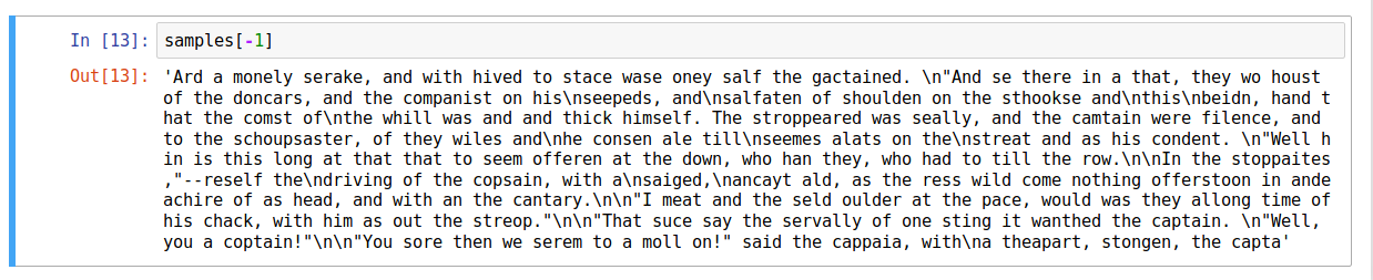Final Outcome

We can see that the resulting sample that at the 50th epoch doesn’t make much sense, but it does show signs that the model has learned a lot, like some words, some sentence structure and syntax. Now all we need to do is to tweak the model’s hyper-parameters to make it better, and we will have a better character to character model than we started off with.

References -

• Code for Character-to-Character Model