Introduction
Any machine learning task involves three steps - data collection, training and evaluation. However, for training a machine learning model, we cannot use raw data. We need to pre-process the data to some suitable form and extract features which can be used for training the model. In the case of NLP, audio signals are used as data, hence one must be familiar with the various processing techniques specific to the audio data types. One of the state-of-the-art tools for extracting features from an audio signal is MFCCs (Mel-frequency cepstral coefficients), hence we will be specifically focusing on MFCC feature extraction.
Useful Techniques and Terminologies
Fourier Transform
Fourier transform is an important tool used in signal processing, it is a mathematical transform that converts a time-domain signal into a frequency domain signal. When we calculate a Fourier transform, we begin with a function of time, f(t), and through mathematical decomposition, we produce a function of frequency, F(ω). When discrete signals are involved, Discrete Fourier Transform (DFT) is used, which is normally computed using the so-called Fast Fourier Transform (FFT). Here is a sample Python code to calculate FFT of an audio clip using the SciPy library. You can refer to this link to know more about FFT.
import numpy as np
from scipy.io import wavfile as wav
from scipy.fft import fft

rate, data = wav.read('audio.wav')
fft_out = fft(data)
print(fft_out)
Spectrum and Cepstrum
Two important features in audio processing are Spectrum and Cepstrum. Both Spectrum and Cepstrum are closely related to each other.
- A spectrum is the Fourier transform of a signal, hence a spectrum is the frequency domain representation of a time-domain audio signal.
- A cepstrum is defined as the Fourier transform of the logarithm of the spectrum. This results in a signal that’s neither in the frequency domain nor in the time domain. The domain of the resulting signal is called the quefrency. You can refer to this link to know more about cepstrum and quefrency.
The reason for converting signals into their frequency domain is related closely to the biology of the human ear. The cochlea is a portion of the inner ear that looks like a snail shell and is a fluid-filled part with thousands of tiny hairs that are connected to nerves. The shorter hairs resonate with higher frequencies and the longer hairs resonate with lower frequencies. Since our ears are frequency analyzers, decomposing audio signals into frequency domain seems like a logical approach to extract features from it.
The Mel-Frequency Scale
The human hearing is highly selective to lower frequencies ( < 1000 Hz) and this keeps decreasing as the frequency increases. Mel-Frequency Scale is a kind of psycho-acoustic scale, derived from a set of experiments on human subjects. It has high resolution at lower frequencies and the resolution keeps decreasing as the frequency increases, hence it helps to simulate the way human ears work.
Mel-frequency cepstral coefficients (MFCC)
One popular audio feature extraction method is the Mel-frequency cepstral coefficients (MFCC). They are coefficients that collectively make up an MFC (Mel-frequency cepstrum). In the MFC, the frequency bands are equally spaced on the Mel scale, which approximates the human auditory system’s response more closely than the linearly-spaced frequency bands used in the normal cepstrum. Hence MFCCs can represent human audio signals more effectively as compared to ordinary cepstrum or other transformations.
Steps to calculate Mel-frequency cepstral coefficients
- Break the signal into overlapping frames.
- Apply FFT to get the frequency Spectrum.
- Apply Mel Filter banks.
- Take the logarithm.
- Apply FFT to get the Mel-frequency cepstral coefficients.
- Keep the first 13 coefficients and discard the rest.
Calculating MFCC in Python
Howevere there are many wonderful libraries in python which can do all this in a single line of code. One such library is Librosa. The code for generating MFCC for a sample audio clip is given below.
import librosa
from librosa import display
import matplotlib.pyplot as plt
y, sr = librosa.load(librosa.util.example_audio_file()) # reading audio clip
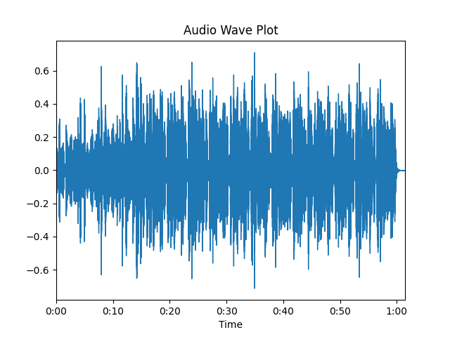
librosa.display.waveplot(y, sr=sr) # plotting audio clip
plt.title('Audio Wave Plot')
plt.show()
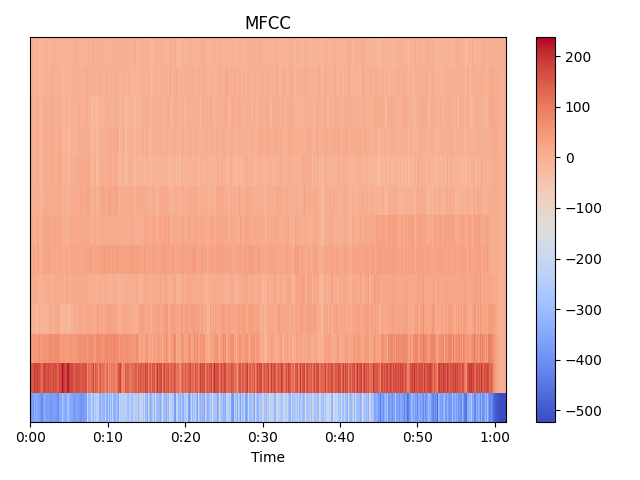
mfccs = librosa.feature.mfcc(y=y, sr=sr, n_mfcc=13) # calculating the first 13 MFCCs
librosa.display.specshow(mfccs, x_axis='time') # plotting the MFCCs
plt.colorbar()
plt.title('MFCC')
plt.tight_layout()
plt.show()
This is the wave plot of the sample audio clip.
This is the plot of the first 13 MFCCs of the sample audio clip.
References