COMPLEXITY THEORY
Complexity theory is a field focusing on classifying computational problems based on the resources utilized, and relating these classes to each other. Complexity of a problem refers to the amount of resources utilized by it. A computational problem is one which can be solved by the mechanical and electronic implementation of mathematical steps. To accomplish this, we need an algorithm, which is a step-by-step procedure to solve a problem. Complexity theory deals with the complexity of problems which can’t get a better complexity regardless of the algorithm used for solving it.
Resources that a computational problem might require:
- Computation time- depends on various factors such as the CPU clock cycle speed, Algorithm used, Computer Architecture and Organisation.
- Number of system level steps it takes to solve the problem – Depends on the Instruction Set Architecture of the sytem.
- Memory Space
- Storage
It is generally noticed that as the input size of a problem gets larger, the resources utilized by the problem also increase. Taking all the above mentioned resources into account and the fact that the resource utilization depends on the input size, a tool was developed to effectively represent the complexity of an algorithm as a function of its input size called – the asymptotic notation
ASYMPTOTIC NOTATION
While defining the asymptotic running time of an algorithm, we assume that the input size is always given as an integer value. In other words, the domain of any function that defines the running time of an algorithm is the set of natural numbers (N = {1, 2, 3 ….})
Say T(n) represents the running time of an algorithm, which has been calculated taking all the above mentioned facts into consideration. But the exact running time of an algorithm is of little use to any programmer and it also takes enough time to find it. Instead, we can just know the abstract running time, using which we can easily compare two algorithms and tell which one is better. This is the asymptotic notation, which is applied to running times of algorithms.
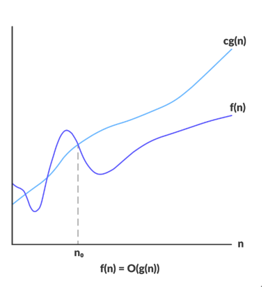
- The Big O notation:
A function f(n) belongs to O(g(n)) if f(n) < cg(n) for some c>0 and all n> some N0. This defines the worst case time of the algorithm.
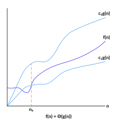
- The Big theta notation:
A function f(n) belongs to Θ(g(n)) if c1g(n) < f(n) < c2g(n) for c1 > 0 and c2 > 0 and all n > some N0. This defines average case time of the algorithm.
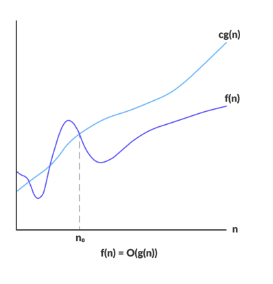
- The Big Omega notation:
A function f(n) belongs to Ω(g(n)) if cg(n) < f(n) for c>0 and all n>some N0. This defines the Best case time of the algorithm.
POLYNOMIAL TIME
Polynomial time or polytime is the time represented by O(nk), i.e. any problem whose worst case running time is of the order of nk is said to execute in polytime.
CLASSES OF COMPUTATIONAL PROBLEMS
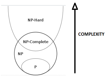
- P class of problems: These are the class of problems which can be solved in polytime, i.e. there exists an algorithm to solve these problems in O(nk)time.
- NP class of problems: These are the class of problems which can be verified in polytime. This means that they may or may not have a polytime solution but given a solution to the problem, it can be verified in polytime whether the solution given is valid or not. Evidently the NP class of problems are decision problems, i.e their output is either yes or no. P is a subset of NP, as any problem that has a polytime solution can also be verified in polytime. Whether it is a proper subset is still an open question.
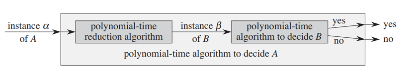
POLYNOMIAL TIME REDUCTIONS
This concept is used to solve problems using the solutions to other problems. If an algorithm to solve one problem is known to us and we need to solve another problem, we can convert/reduce the second problem to an input of the first one and use the output of the first problem hence obtained as the output to the second problem as well. However,

1.  The reduction must be carried out in polytime
2.  The number of times the first problem has to be solved to solve the second one also must be polynomial.

Then the second problem is said to be polytime reducible to the first one. This reduction indicates that the second problem is no harder than the first one, i.e. if we can efficiently solve the first problem we can solve the second one as well.

An instance of a problem is the problem along with its inputs(Say if A is our problem A(a,b,c) where a,b,c are inputs, is an instance). Technically speaking, an instance of problem A has to be reduced to an instance of problem B to solve problem A using B.
- NP-Complete(NPC): These are the class of problems which are also a subset of NP and all problems in the class NP can be polytime reduced to these problems. NPC problems are of great significance as they have the power to answer the “question of the millennium” – is P=NP or P≠NP. This is because, if a polytime algorithm can be generated to solve any of the NPC problems, it would imply that all NP problems can also be solved in polytime, since they are polytime reducible to the NPC problem. Hence P=NP. On the other hand if it can be proved that no polytime algorithm exists for any of the NPC problems, it would also imply that no polytime algorithm exists for any NP problem, i.e. P≠NP.
- NP-hard: NP-hard problems are those which may or may not have a polytime verifier but all NP problems can be polytime reduced to NP-hard problems. NPC = NP Ո NP-hard